Lecture8 (deep_learning_part3_2.pdf, 37 หน้า) · 2603520 Deep Learning

CNN Architectures, Transfer Learning และ Vision Transformers

Lesson 7 ให้ชิ้นส่วนของ CNN (convolution, pooling, การนับ parameter). บทนี้ใช้ชิ้นส่วนเหล่านั้นตอบสามคำถาม:

  1. สถาปัตยกรรมที่มีชื่อแต่ละตัวแก้ปัญหาอะไร (LeNet → AlexNet → VGG → Inception → ResNet → รุ่นใหม่; หน้า 2–20)
  2. จะนำโมเดลที่เทรนแล้วมาใช้กับงานของเราอย่างไร (transfer learning สามแบบ และโค้ด Keras; หน้า 21–29)
  3. ถ้าไม่ใช้ convolution เลยจะได้อะไร (ViT และ Swin Transformer; หน้า 30–37)
อ่านเพิ่มก่อนเริ่ม (แนะนำ)
Keras Applications (รายชื่อ pretrained model พร้อม accuracy และจำนวน parameter; สไลด์หน้า 16 อ้างถึง) · Keras — Transfer learning & fine-tuning · ต้นฉบับ: VGG, ResNet, ViT, Swin.
คำที่ใช้ทั้งบท
ต้องรู้ก่อน — สองสูตรจาก Lesson 7

ทุกการคำนวณในบทนี้ใช้สองสูตรเดิม:

$$\begin{gathered}\text{output size} = \left\lfloor \frac{n + 2p - f}{s} \right\rfloor + 1 \\[0.35em] \\[0.35em] \#\text{param}_{\text{conv}} = (f \cdot f \cdot n_C + 1) \cdot n_C'\end{gathered}$$

และสูตรของ dense layer: \(n_{in} \cdot n_{out} + n_{out}\). สัญลักษณ์ "3 × 3 + 1(S)" ในรูปของสไลด์หมายถึง kernel 3×3, stride 1, padding "same".

1. ILSVRC และแผนที่วิวัฒนาการของ CNN

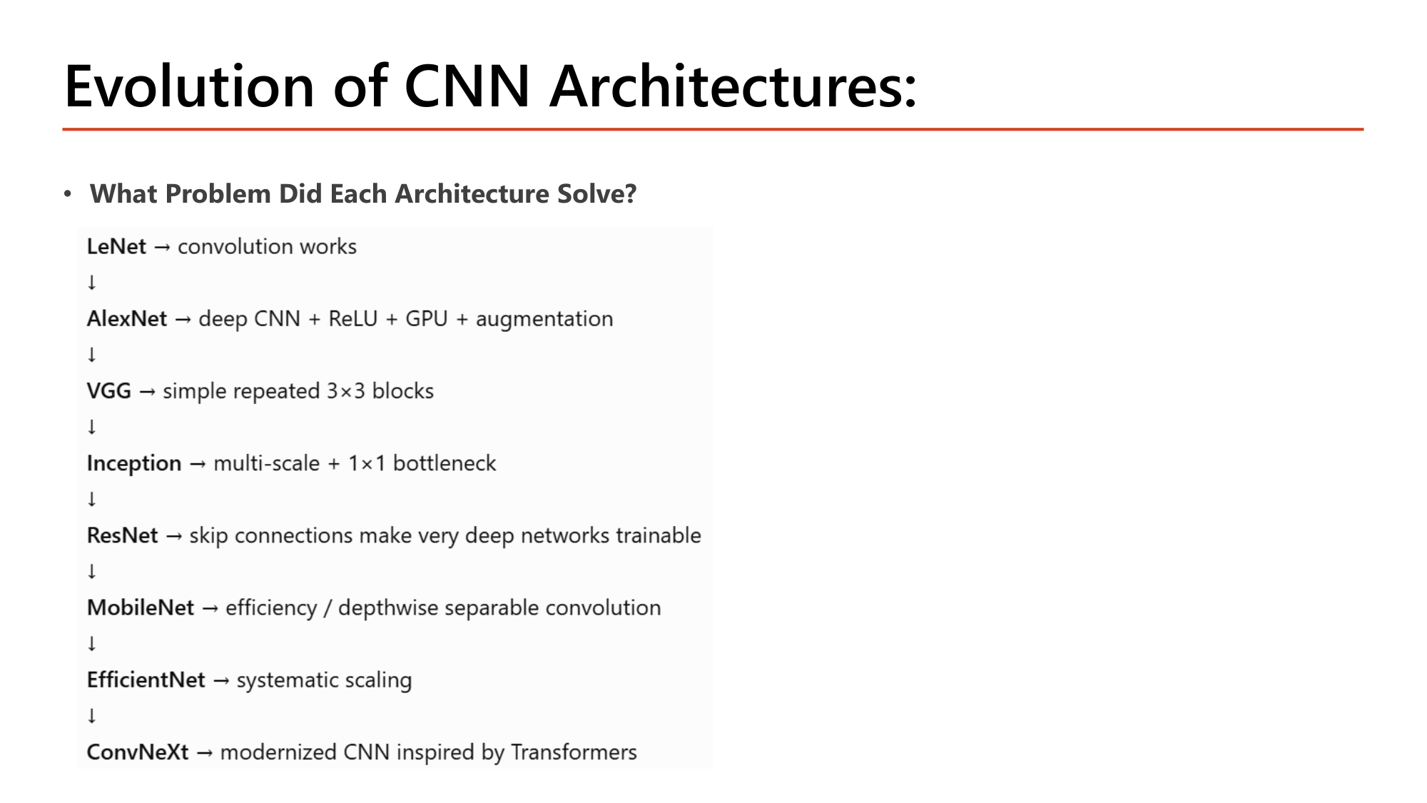
Slide: Evolution of CNN Architectures: What problem did each architecture solve? LeNet: convolution works. AlexNet: deep CNN + ReLU + GPU + augmentation. VGG: simple repeated 3x3 blocks. Inception: multi-scale + 1x1 bottleneck. ResNet: skip connections make very deep networks trainable. MobileNet: efficiency, depthwise separable convolution. EfficientNet: systematic scaling. ConvNeXt: modernized CNN inspired by Transformers
Slide: Evolution of CNN Architectures — แต่ละรุ่นแก้ปัญหาอะไร (Lecture8, p.2)

หน้า 2 คือสารบัญของครึ่งแรกของบท. แต่ละสถาปัตยกรรมมีหนึ่งคำตอบต่อคำถาม "What Problem Did Each Architecture Solve?":

สถาปัตยกรรมสิ่งที่แก้/พิสูจน์ (ตามสไลด์)หัวข้อ
LeNetconvolution works§2
AlexNetdeep CNN + ReLU + GPU + augmentation§3
VGGsimple repeated 3×3 blocks§4
Inceptionmulti-scale + 1×1 bottleneck§5
ResNetskip connections make very deep networks trainable§6
MobileNetefficiency / depthwise separable convolution§7
EfficientNetsystematic scaling§7
ConvNeXtmodernized CNN inspired by Transformers§7
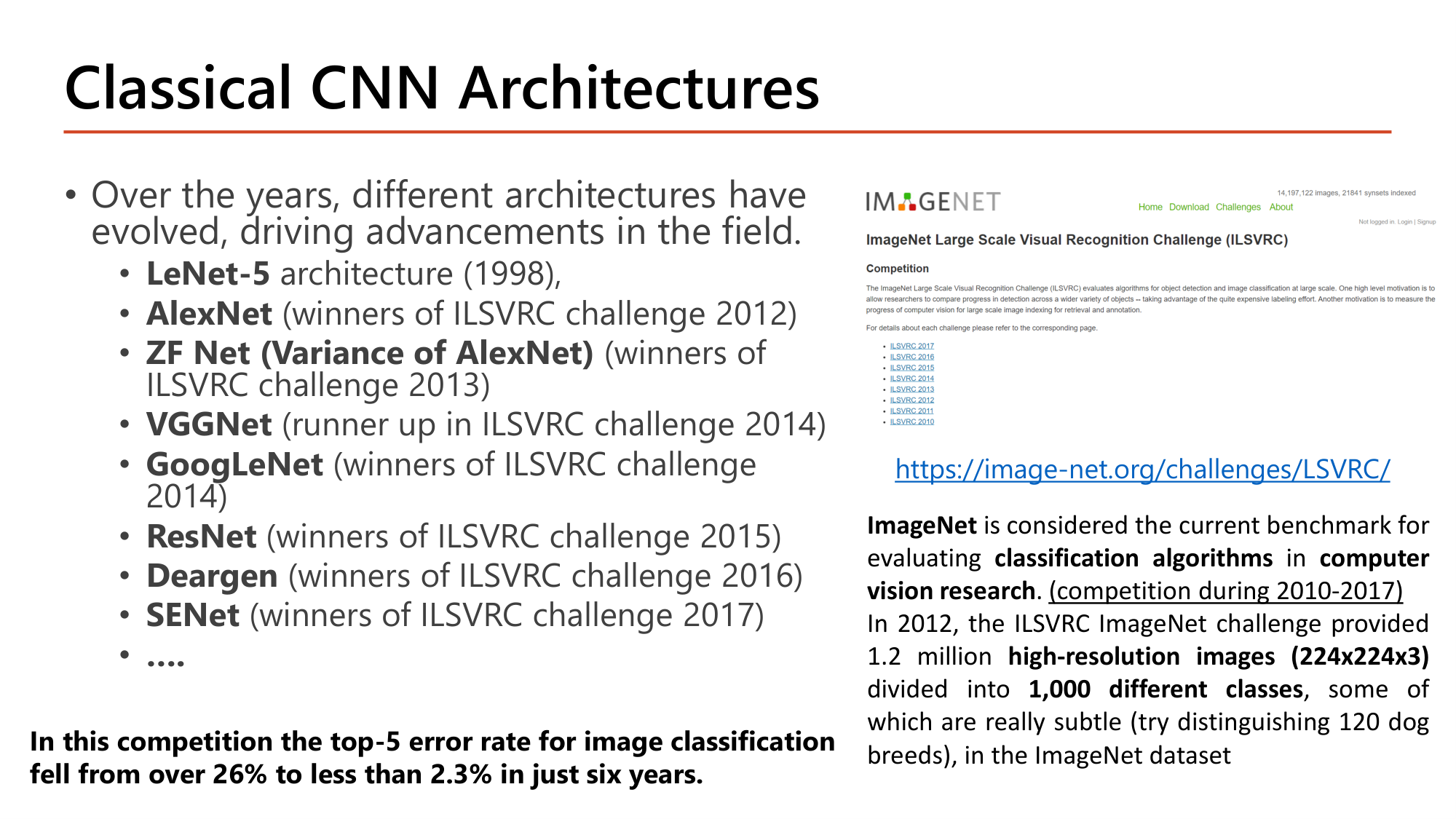
Slide: Classical CNN Architectures. LeNet-5 (1998), AlexNet (winner ILSVRC 2012), ZF Net (2013), VGGNet (runner up 2014), GoogLeNet (winner 2014), ResNet (winner 2015), 2016 winner, SENet (winner 2017). ImageNet is the benchmark for classification algorithms (competition 2010-2017). In 2012 ILSVRC provided 1.2 million high-resolution images (224x224x3) in 1,000 classes. Top-5 error rate fell from over 26% to less than 2.3% in six years
Slide: Classical CNN Architectures — ผู้ชนะ ILSVRC (Lecture8, p.3)

ImageNet เป็น benchmark สำหรับประเมินอัลกอริทึมจำแนกภาพ (การแข่งขันจัดช่วงปี 2010–2017). ในปี 2012 ILSVRC ให้ภาพความละเอียดสูง 1.2 ล้านภาพ (224×224×3) แบ่งเป็น 1,000 class ซึ่งบาง class ต่างกันน้อยมาก (เช่น สุนัข 120 สายพันธุ์). ตัวเลขสำคัญของสไลด์: top-5 error rate ลดจากมากกว่า 26% เหลือน้อยกว่า 2.3% ภายในหกปี.

ปีสถาปัตยกรรมผล ILSVRC
1998LeNet-5(ก่อนมีการแข่งขัน)
2012AlexNetwinner
2013ZF Net (variance ของ AlexNet)winner
2014VGGNetrunner up
2014GoogLeNetwinner
2015ResNetwinner
2017SENetwinner
คำถาม 1Top-5 error
โมเดลหนึ่งทดสอบกับภาพ 2,000 ภาพ โดยมี 1,500 ภาพที่ class จริงเป็นอันดับ 1 ของคำทำนาย และอีก 380 ภาพที่ class จริงอยู่อันดับ 2 ถึง 5 top-5 error rate ของโมเดลนี้คือเท่าใด?

2. LeNet-5 (1998): convolution ใช้ได้จริง

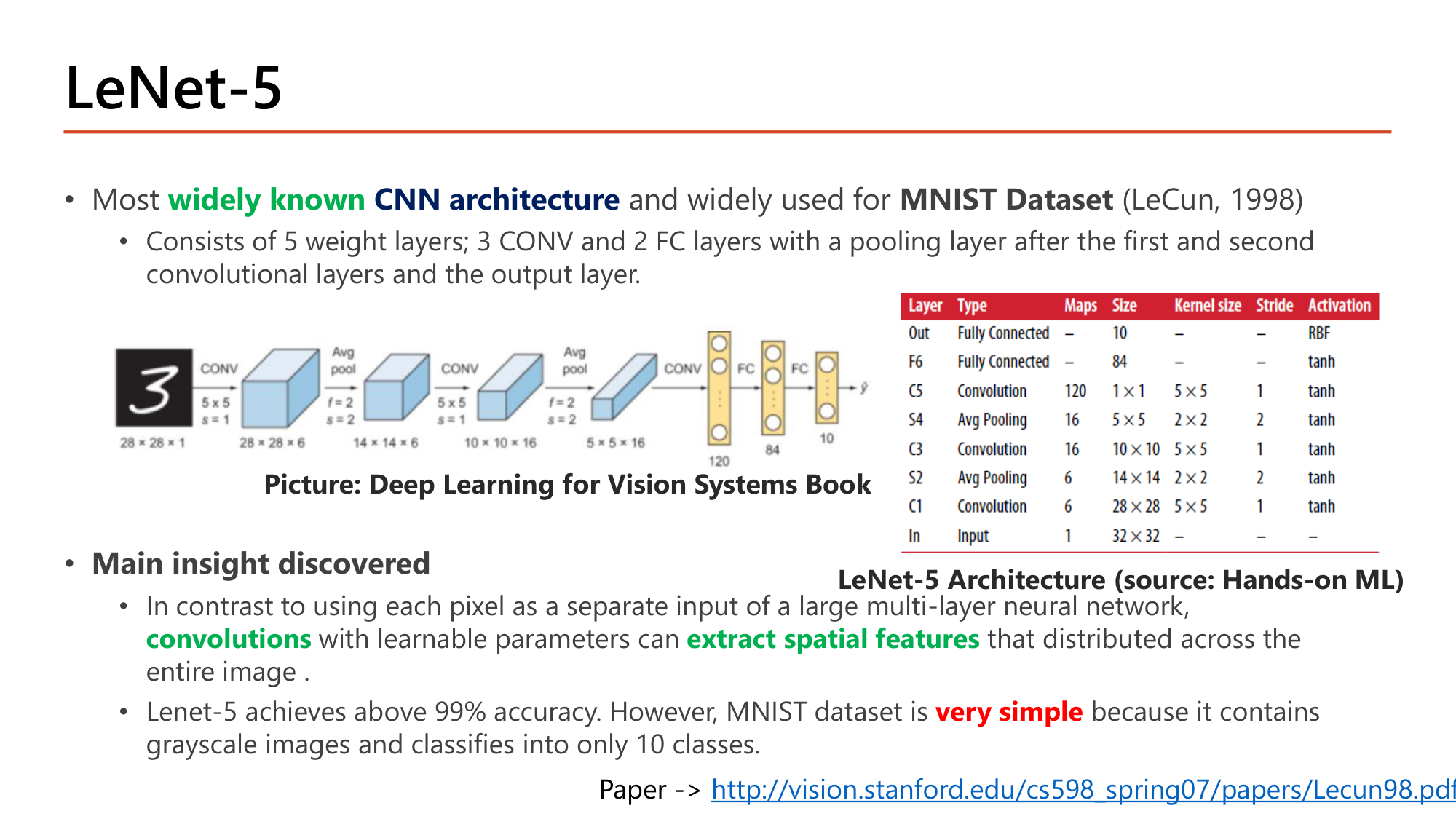
Slide: LeNet-5. Most widely known CNN architecture, widely used for MNIST (LeCun, 1998). 5 weight layers: 3 CONV and 2 FC, with a pooling layer after the first and second convolutional layers. Main insight: convolutions with learnable parameters can extract spatial features distributed across the entire image. Achieves above 99% accuracy, but MNIST is very simple (grayscale, 10 classes). Diagram 28x28x1, 28x28x6, 14x14x6, 10x10x16, 5x5x16, 120, 84, 10 and a layer table with tanh activations and average pooling
Slide: LeNet-5 — 3 CONV + 2 FC (Lecture8, p.4)

LeNet-5 เป็น CNN architecture ที่ widely known ที่สุด และใช้กับ MNIST (LeCun, 1998). ประกอบด้วย 5 weight layers: 3 CONV และ 2 FC โดยมี pooling หลัง CONV ชั้นที่หนึ่งและสอง. ตารางในสไลด์ระบุว่าใช้ average pooling และ activation tanh (ไม่ใช่ max pooling และ ReLU แบบปัจจุบัน).

Main insight discovered: แทนที่จะใช้แต่ละ pixel เป็น input แยกกันของ network ขนาดใหญ่ convolutions ที่มี learnable parameters สามารถ extract spatial features ที่กระจายอยู่ทั่วทั้งภาพ. LeNet-5 ได้ accuracy สูงกว่า 99% แต่ MNIST เป็น dataset ที่ very simple เพราะเป็นภาพ grayscale และมีเพียง 10 class.

คำนวณตามรูปในสไลด์: shape และ parameter ของ LeNet-5
ให้ input 28×28×1. CONV ทุกชั้นใช้ kernel 5×5 stride 1. Pooling ใช้ f = 2, s = 2. CONV ชั้นแรก padding same; ชั้นที่เหลือ padding valid
  1. ขั้นที่ 1 — CONV1 (6 filter, same) และ POOL
    $$\begin{gathered}28 \times 28 \times 6,\quad (5 \cdot 5 \cdot 1 + 1) \cdot 6 = 156 \\[0.35em] \Rightarrow\; 14 \times 14 \times 6\end{gathered}$$
  2. ขั้นที่ 2 — CONV2 (16 filter, valid) และ POOL
    $$\begin{gathered}14 - 5 + 1 = 10 \;\Rightarrow\; 10 \times 10 \times 16 \\[0.35em] (5 \cdot 5 \cdot 6 + 1) \cdot 16 = 2{,}416 \\[0.35em] \rightarrow\; 5 \times 5 \times 16\end{gathered}$$
  3. ขั้นที่ 3 — CONV3 (120 filter, valid)
    $$\begin{gathered}5 - 5 + 1 = 1 \;\Rightarrow\; 1 \times 1 \times 120\\ (5 \cdot 5 \cdot 16 + 1) \cdot 120 = 48{,}120\end{gathered}$$
  4. ขั้นที่ 4 — FC 84 node และ output 10 node
    $$120 \times 84 + 84 = 10{,}164 \qquad 84 \times 10 + 10 = 850$$
  5. ขั้นที่ 5 — รวม
    $$156 + 2{,}416 + 48{,}120 + 10{,}164 + 850 = 61{,}706$$

LeNet-5 มีราว 62,000 parameter. ตารางจาก Hands-on ML ในสไลด์ใช้ input 32×32 และ padding valid ทุกชั้น จึงได้ 32 → 28 → 14 → 10 → 5 → 1 ซึ่งลงท้ายที่ขนาดเดียวกัน.
ออกสอบสูง — ข้อความที่อาจารย์ทำสี

3. AlexNet (2012): ลึกขึ้น ใหญ่ขึ้น

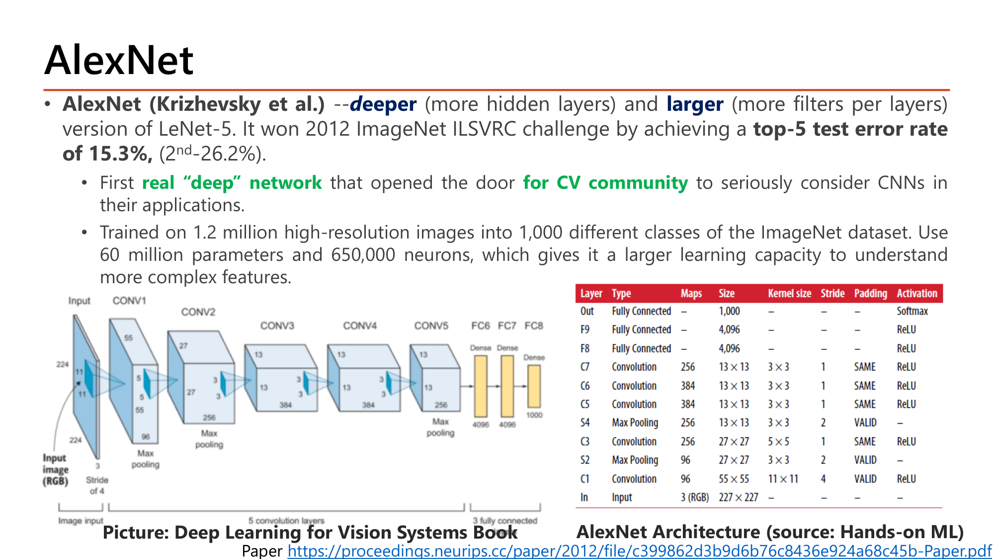
Slide: AlexNet (Krizhevsky et al.), a deeper (more hidden layers) and larger (more filters per layer) version of LeNet-5. Won ILSVRC 2012 with top-5 test error 15.3% (2nd place 26.2%). First real deep network that opened the door for the CV community. Trained on 1.2 million images in 1,000 classes; 60 million parameters and 650,000 neurons. Layer table: input 227x227x3, C1 96 maps 55x55 kernel 11x11 stride 4 valid, S2 max pool 27x27, C3 256 maps kernel 5x5 same, S4 13x13, C5 384, C6 384, C7 256 kernel 3x3 same, F8 4096, F9 4096, Out 1000 softmax
Slide: AlexNet — สถาปัตยกรรมและตาราง layer (Lecture8, p.5)

AlexNet (Krizhevsky et al.) คือ LeNet-5 รุ่นที่ deeper (hidden layer มากขึ้น) และ larger (filter ต่อ layer มากขึ้น). ชนะ ILSVRC 2012 ด้วย top-5 test error rate 15.3% ขณะที่อันดับสองได้ 26.2%. เป็น real “deep” network ตัวแรกที่เปิดทาง for CV community ให้พิจารณา CNN อย่างจริงจัง. เทรนบนภาพ 1.2 ล้านภาพ 1,000 class ใช้ 60 million parameters และ 650,000 neurons.

คำนวณตามตารางในสไลด์: ขนาด feature map ของ AlexNet และที่อยู่ของ parameter
ให้ input 227×227×3 (ค่าในตารางของสไลด์)
  1. ขั้นที่ 1 — C1: 96 filter, 11×11, stride 4, valid
    $$\begin{gathered}\left\lfloor \frac{227 - 11}{4} \right\rfloor + 1 = 54 + 1 = 55 \\[0.35em] \#\text{param} = (11 \cdot 11 \cdot 3 + 1) \cdot 96 = 34{,}944\end{gathered}$$
  2. ขั้นที่ 2 — S2: max pool 3×3, stride 2
    $$\left\lfloor \frac{55 - 3}{2} \right\rfloor + 1 = 27$$
  3. ขั้นที่ 3 — C3 (256 filter, 5×5, same) คงขนาด 27; S4: max pool 3×3, stride 2
    $$\left\lfloor \frac{27 - 3}{2} \right\rfloor + 1 = 13$$
  4. ขั้นที่ 4 — C5, C6, C7 (384, 384, 256 filter, 3×3, same) คงขนาด 13; max pool สุดท้าย
    $$\begin{gathered}\left\lfloor \frac{13 - 3}{2} \right\rfloor + 1 = 6 \\[0.35em] \Rightarrow\; 6 \times 6 \times 256 = 9{,}216\end{gathered}$$
  5. ขั้นที่ 5 — F8: dense 4,096 node
    $$9{,}216 \times 4{,}096 + 4{,}096 = 37{,}752{,}832$$

ลำดับขนาด 227 → 55 → 27 → 13 → 6 ตรงกับคอลัมน์ Size ของตาราง. Dense layer ชั้นเดียว (F8) มี 37.8 ล้าน parameter จากทั้งหมดราว 62 ล้าน คือมากกว่าครึ่ง ส่วน C1 มีเพียง 34,944. โค้ดในหน้า 6 ใช้ input_shape=(224,224,3) ซึ่งให้ \(\lfloor 213/4 \rfloor + 1 = 54\) สไลด์จึงกำกับว่า "not totally similar to original".
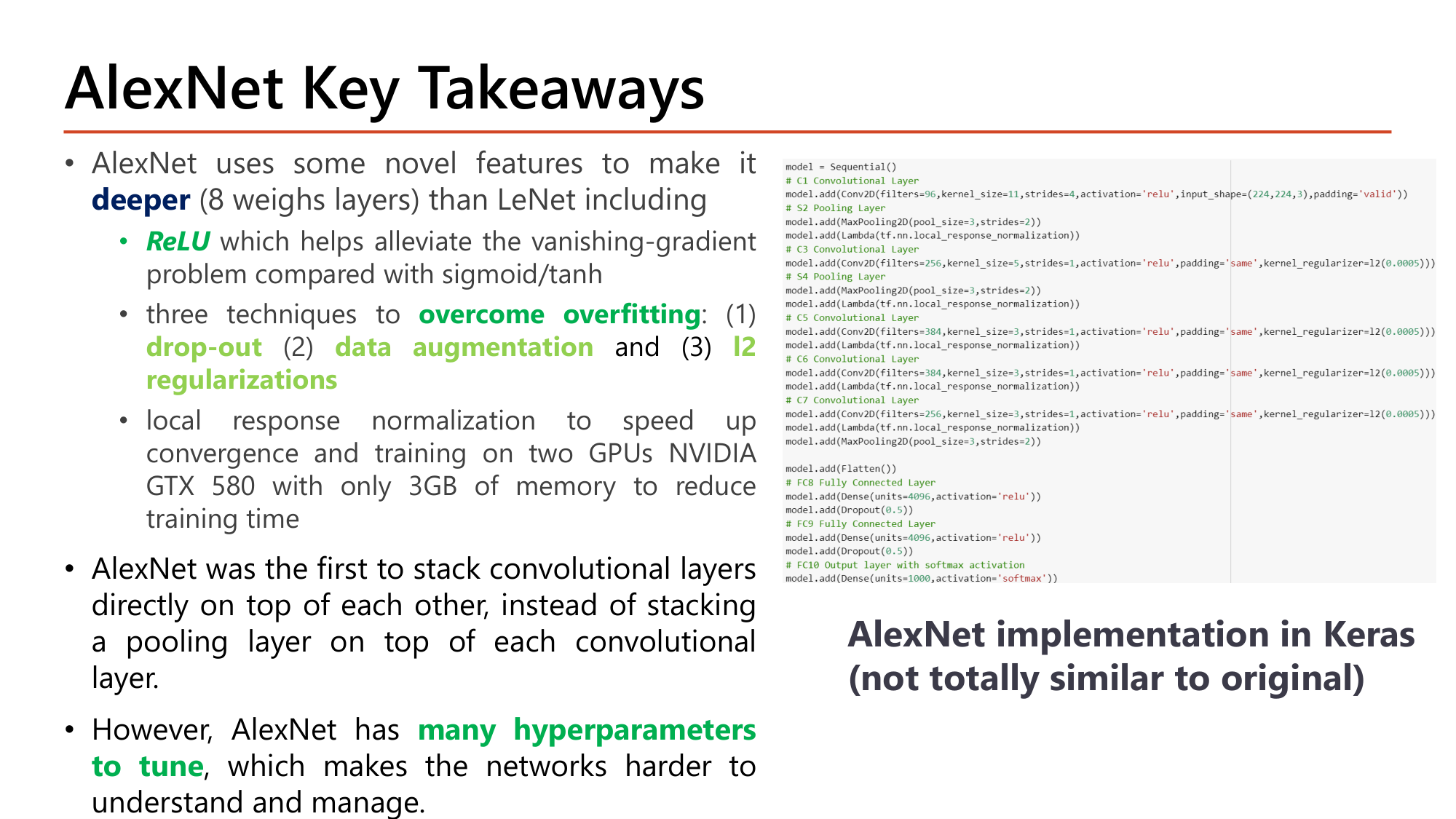
Slide: AlexNet Key Takeaways. Novel features to make it deeper (8 weight layers) than LeNet: ReLU which alleviates vanishing gradient compared with sigmoid/tanh; three techniques to overcome overfitting: dropout, data augmentation, L2 regularization; local response normalization and training on two GTX 580 GPUs with 3GB memory. First to stack convolutional layers directly on top of each other. However, AlexNet has many hyperparameters to tune. Keras implementation code shown
Slide: AlexNet Key Takeaways — พร้อมโค้ด Keras (Lecture8, p.6)

AlexNet ใช้เทคนิคใหม่หลายอย่างเพื่อให้ deeper (8 weight layers: 5 CONV + 3 FC) กว่า LeNet:

ข้อเสีย: AlexNet มี many hyperparameters to tune (kernel 11, 5, 3; stride 4, 1; padding valid/same ต่างกันทุกชั้น) ทำให้เข้าใจและจัดการยาก. ข้อเสียนี้คือโจทย์ที่ VGG แก้ใน §4.

model = Sequential()
# C1 Convolutional Layer
model.add(Conv2D(filters=96,kernel_size=11,strides=4,activation='relu',input_shape=(224,224,3),padding='valid'))
# S2 Pooling Layer
model.add(MaxPooling2D(pool_size=3,strides=2))
model.add(Lambda(tf.nn.local_response_normalization))
# C3 Convolutional Layer
model.add(Conv2D(filters=256,kernel_size=5,strides=1,activation='relu',padding='same',kernel_regularizer=l2(0.0005)))
# S4 Pooling Layer
model.add(MaxPooling2D(pool_size=3,strides=2))
model.add(Lambda(tf.nn.local_response_normalization))
# C5 Convolutional Layer
model.add(Conv2D(filters=384,kernel_size=3,strides=1,activation='relu',padding='same',kernel_regularizer=l2(0.0005)))
model.add(Lambda(tf.nn.local_response_normalization))
# C6 Convolutional Layer
model.add(Conv2D(filters=384,kernel_size=3,strides=1,activation='relu',padding='same',kernel_regularizer=l2(0.0005)))
model.add(Lambda(tf.nn.local_response_normalization))
# C7 Convolutional Layer
model.add(Conv2D(filters=256,kernel_size=3,strides=1,activation='relu',padding='same',kernel_regularizer=l2(0.0005)))
model.add(Lambda(tf.nn.local_response_normalization))
model.add(MaxPooling2D(pool_size=3,strides=2))

model.add(Flatten())
# FC8 Fully Connected Layer
model.add(Dense(units=4096,activation='relu'))
model.add(Dropout(0.5))
# FC9 Fully Connected Layer
model.add(Dense(units=4096,activation='relu'))
model.add(Dropout(0.5))
# FC10 Output layer with softmax activation
model.add(Dense(units=1000,activation='softmax'))
โค้ดทำอะไร
Conv2D(filters=96, kernel_size=11, strides=4, activation='relu', input_shape=(224,224,3), padding='valid')C1: kernel ใหญ่ 11×11 ก้าวทีละ 4 ย่อภาพอย่างรวดเร็วในชั้นแรก. activation เป็น ReLU
MaxPooling2D(pool_size=3, strides=2)หน้าต่าง 3×3 ก้าว 2 ⇒ หน้าต่างซ้อนกัน 1 pixel (overlapping pooling)
Lambda(tf.nn.local_response_normalization)ห่อฟังก์ชันของ TensorFlow เป็น layer ด้วย Lambda. ทำ local response normalization
Conv2D(filters=256, kernel_size=5, ..., padding='same', kernel_regularizer=l2(0.0005))C3: kernel_regularizer=l2(0.0005) คือ L2 regularization บน weight ของ filter (เทคนิคที่ 3)
Conv2D(384, 3) → Conv2D(384, 3) → Conv2D(256, 3)C5–C7: convolution สามชั้นต่อกันโดยไม่มี pooling คั่น
Flatten()แปลง feature map เป็น vector ก่อนเข้า FC
Dense(units=4096, activation='relu') + Dropout(0.5)FC8, FC9: dropout rate 0.5 หลัง dense แต่ละชั้น (เทคนิคที่ 1) อยู่ในส่วน classification
Dense(units=1000, activation='softmax')FC10: 1,000 class ของ ImageNet
คำถาม 2AlexNet
ข้อใดคือชุดเทคนิคสามอย่างที่ AlexNet ใช้เพื่อลด overfitting?
คำถาม 3Output size
Convolution layer แรกของ network หนึ่งรับภาพ 99×99×3 ใช้ 32 filter ขนาด 7×7 stride 4 padding valid shape ของ output คือข้อใด?
ออกสอบสูง — ข้อความที่อาจารย์ทำสี

4. VGGNet (2014): บล็อก 3×3 ซ้ำกันทั้ง network

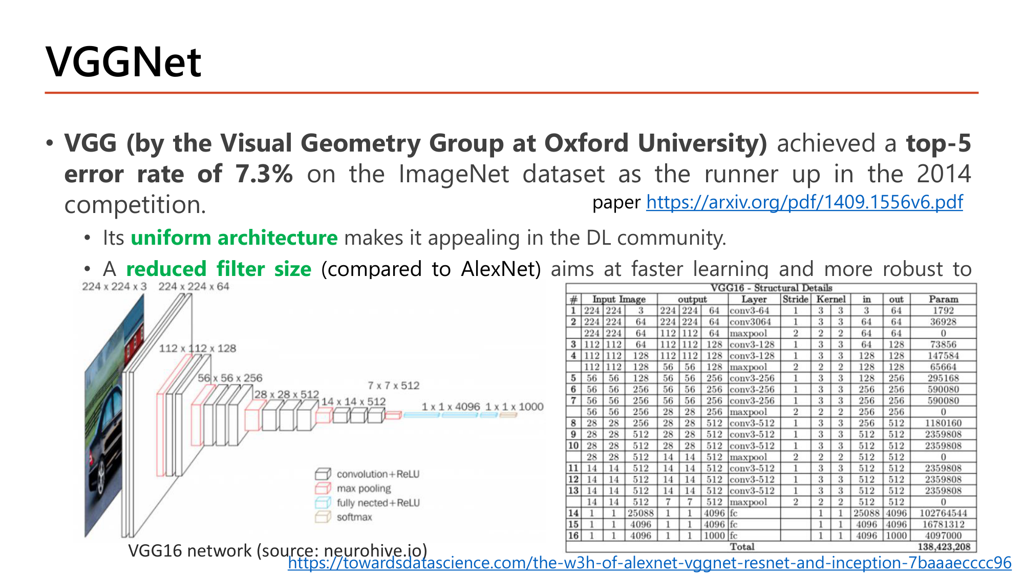
Slide: VGGNet (Visual Geometry Group, Oxford) achieved a top-5 error rate of 7.3% on ImageNet as runner up in 2014. Its uniform architecture makes it appealing. A reduced filter size (compared to AlexNet) aims at faster learning and more robust to overfitting. VGG16 diagram: 224x224x3, 224x224x64, 112x112x128, 56x56x256, 28x28x512, 14x14x512, 7x7x512, 4096, 4096, 1000; structural details table with parameters per layer
Slide: VGGNet — VGG16 (Lecture8, p.7)

VGG (Visual Geometry Group, Oxford University) ได้ top-5 error rate 7.3% เป็น runner up ปี 2014. จุดเด่นคือ uniform architecture และ reduced filter size (เทียบกับ AlexNet) เพื่อให้เรียนเร็วขึ้นและทนต่อ overfitting มากขึ้น. รูป VGG16 แสดงรูปแบบที่สม่ำเสมอ: ทุกครั้งที่ pooling ลดด้านลงครึ่ง จำนวน channel เพิ่มสองเท่า: 224×224×64 → 112×112×128 → 56×56×256 → 28×28×512 → 14×14×512 → 7×7×512 แล้วต่อด้วย FC 4096, 4096, 1000.
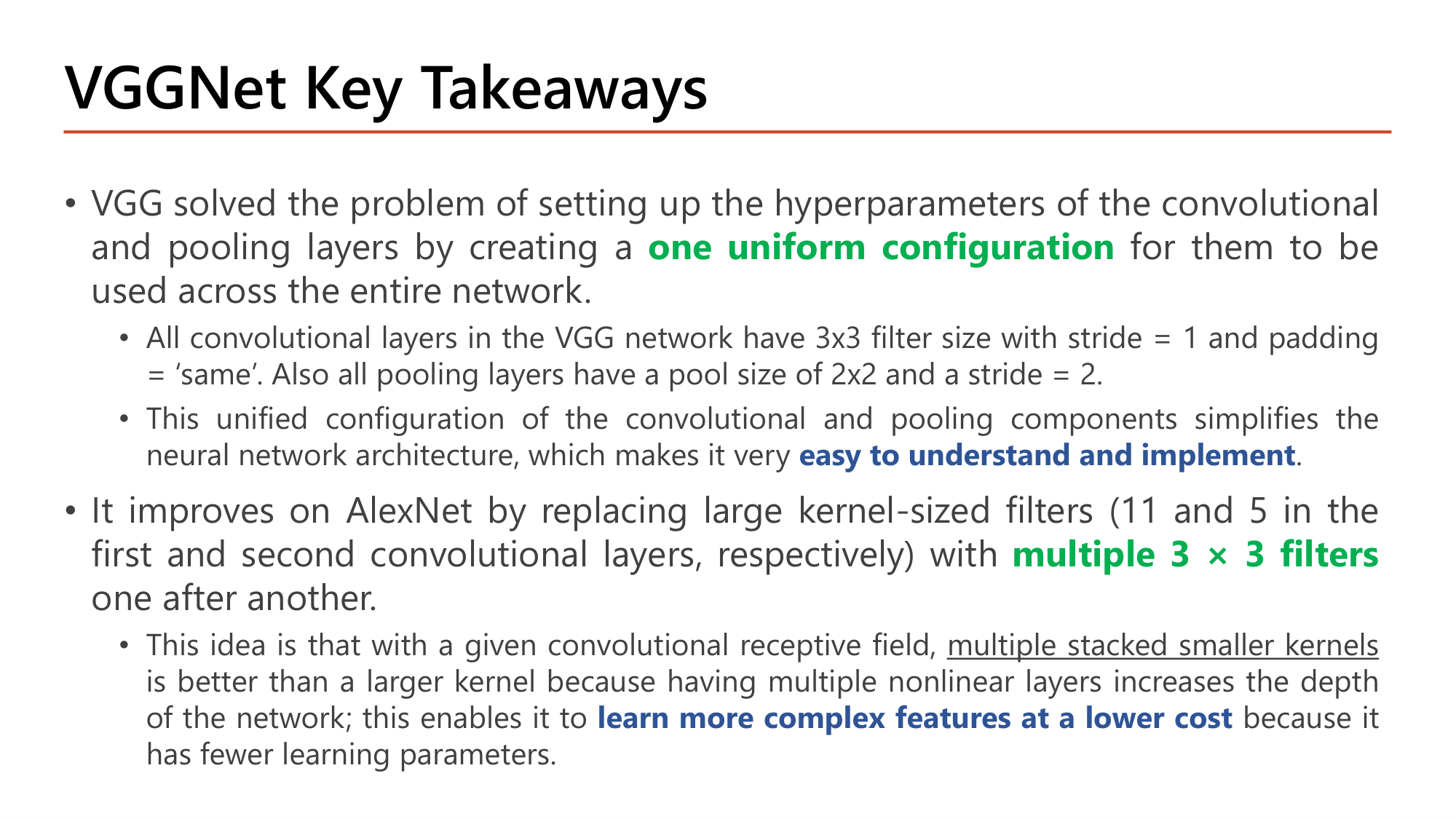
Slide: VGGNet Key Takeaways. VGG solved the problem of setting up hyperparameters of conv and pooling layers by creating one uniform configuration across the entire network: all conv layers 3x3 filter, stride 1, padding same; all pooling layers pool size 2x2, stride 2. This makes it easy to understand and implement. It improves on AlexNet by replacing large kernel-sized filters (11 and 5) with multiple 3x3 filters one after another; multiple stacked smaller kernels is better than a larger kernel: more nonlinear layers, learn more complex features at a lower cost because of fewer parameters
Slide: VGGNet Key Takeaways (Lecture8, p.8)

VGG แก้ปัญหาการตั้ง hyperparameter ของ convolutional และ pooling layer ด้วย one uniform configuration ที่ใช้ทั้ง network:

การกำหนดค่าแบบเดียวนี้ทำให้สถาปัตยกรรม easy to understand and implement. VGG ปรับปรุง AlexNet โดยแทน filter ขนาดใหญ่ (11 และ 5 ในสองชั้นแรก) ด้วย multiple 3 × 3 filters ต่อกัน. เหตุผลในสไลด์: ที่ receptive field เท่ากัน multiple stacked smaller kernels ดีกว่า kernel ใหญ่ตัวเดียว เพราะมี nonlinear layer หลายชั้นจึงเพิ่มความลึก ทำให้ learn more complex features at a lower cost จากการที่มี parameter น้อยกว่า.

คำนวณ: 3×3 สองชั้นเทียบกับ 5×5 หนึ่งชั้น
ให้ input และ output มี 64 channel ทุกชั้น, stride 1
  1. ขั้นที่ 1 — Receptive field ของ 3×3 ซ้อนสองชั้น

    output หนึ่งค่าของชั้นที่สองมองเห็น 3×3 ค่าของชั้นแรก และแต่ละค่านั้นมองเห็น 3×3 pixel ที่เหลื่อมกันทีละ 1

    $$3 + (3 - 1) = 5 \quad\Rightarrow\quad 5 \times 5$$
  2. ขั้นที่ 2 — Parameter ของ 5×5 หนึ่งชั้น
    $$(5 \cdot 5 \cdot 64 + 1) \cdot 64 = 102{,}464$$
  3. ขั้นที่ 3 — Parameter ของ 3×3 สองชั้น
    $$2 \times (3 \cdot 3 \cdot 64 + 1) \cdot 64 = 2 \times 36{,}928 = 73{,}856$$
  4. ขั้นที่ 4 — กรณี 7×7: 3×3 สามชั้นให้ receptive field \(3 + 2 + 2 = 7\)
    $$(7 \cdot 7 \cdot 64 + 1) \cdot 64 = 200{,}768 \qquad 3 \times 36{,}928 = 110{,}784$$

Receptive field เท่ากัน แต่ 3×3 สองชั้นใช้ parameter น้อยกว่า 28% (73,856 เทียบกับ 102,464) และมี ReLU สองครั้งแทนหนึ่งครั้ง. กรณี 7×7 ประหยัดได้ 45%. ค่า 36,928 คือค่าที่ปรากฏในตาราง VGG16 ของสไลด์สำหรับ conv ชั้นที่สอง.
คำถาม 4VGG
ข้อใดคือ configuration ที่ VGG ใช้เหมือนกันทั้ง network?
คำถาม 5VGG
Convolution 3×3 ซ้อนกันสามชั้น (stride 1) มี receptive field เทียบเท่า convolution ชั้นเดียวขนาดใด และถ้าทุกชั้นมี 32 channel (ไม่นับ bias) แบบใดใช้ weight น้อยกว่า?
ออกสอบสูง — ข้อความที่อาจารย์ทำสี

5. Inception และ GoogLeNet (2014): หลายขนาด filter พร้อมกัน + 1×1 bottleneck

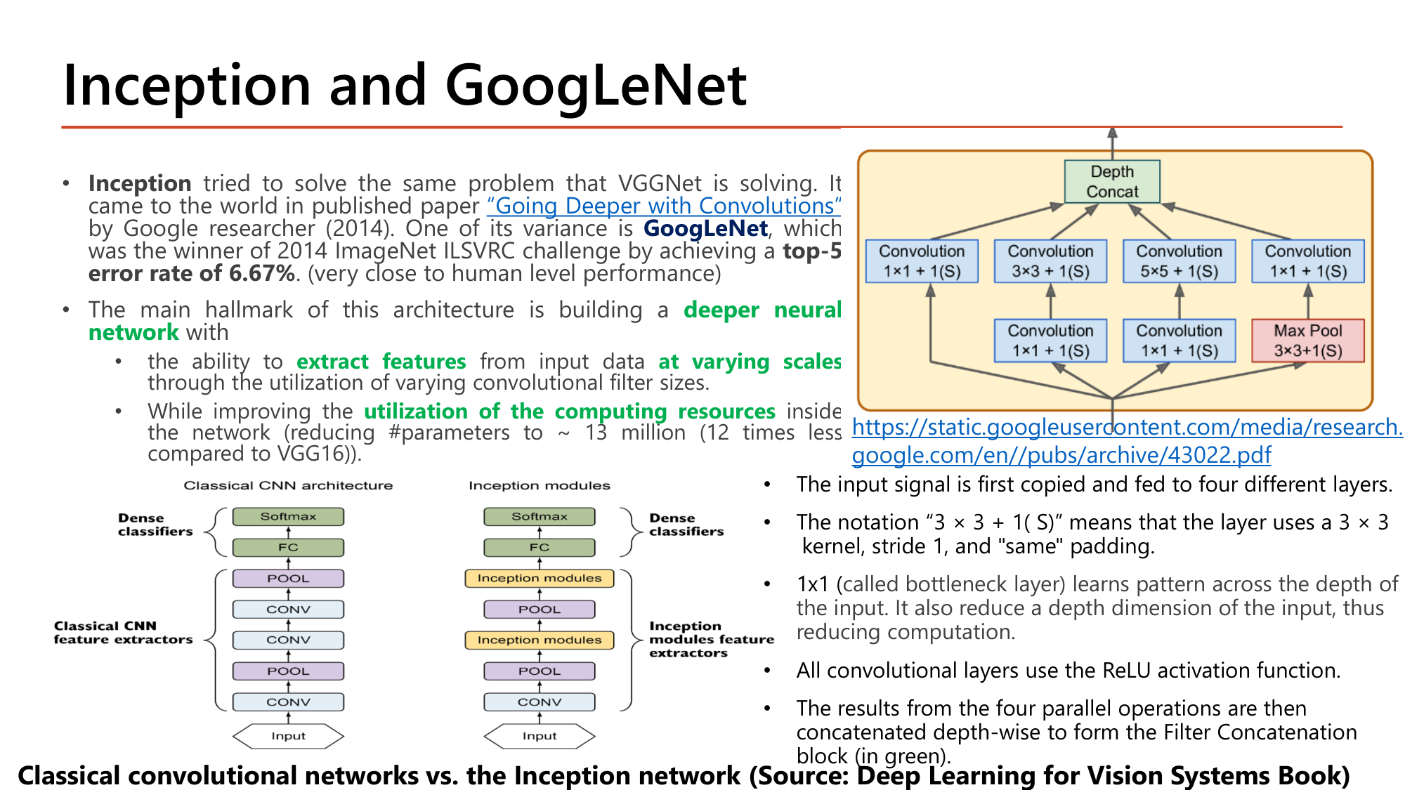
Slide: Inception and GoogLeNet. Inception tried to solve the same problem as VGGNet (paper Going Deeper with Convolutions, Google, 2014). GoogLeNet won ILSVRC 2014 with top-5 error 6.67%. Hallmark: a deeper neural network with the ability to extract features at varying scales through varying convolutional filter sizes, while improving utilization of computing resources (about 13 million parameters, 12 times less than VGG16). Inception module diagram: input copied to four branches: 1x1 conv; 1x1 then 3x3; 1x1 then 5x5; 3x3 max pool then 1x1; depth concat
Slide: Inception and GoogLeNet — inception module (Lecture8, p.9)

Inception แก้โจทย์เดียวกับ VGGNet. เผยแพร่ในบทความ "Going Deeper with Convolutions" ของนักวิจัย Google (2014). รุ่นหนึ่งคือ GoogLeNet ซึ่งชนะ ILSVRC 2014 ด้วย top-5 error rate 6.67% (ใกล้ระดับมนุษย์). เอกลักษณ์คือการสร้าง deeper neural network ที่

การทำงานของ inception module ตามรูป:
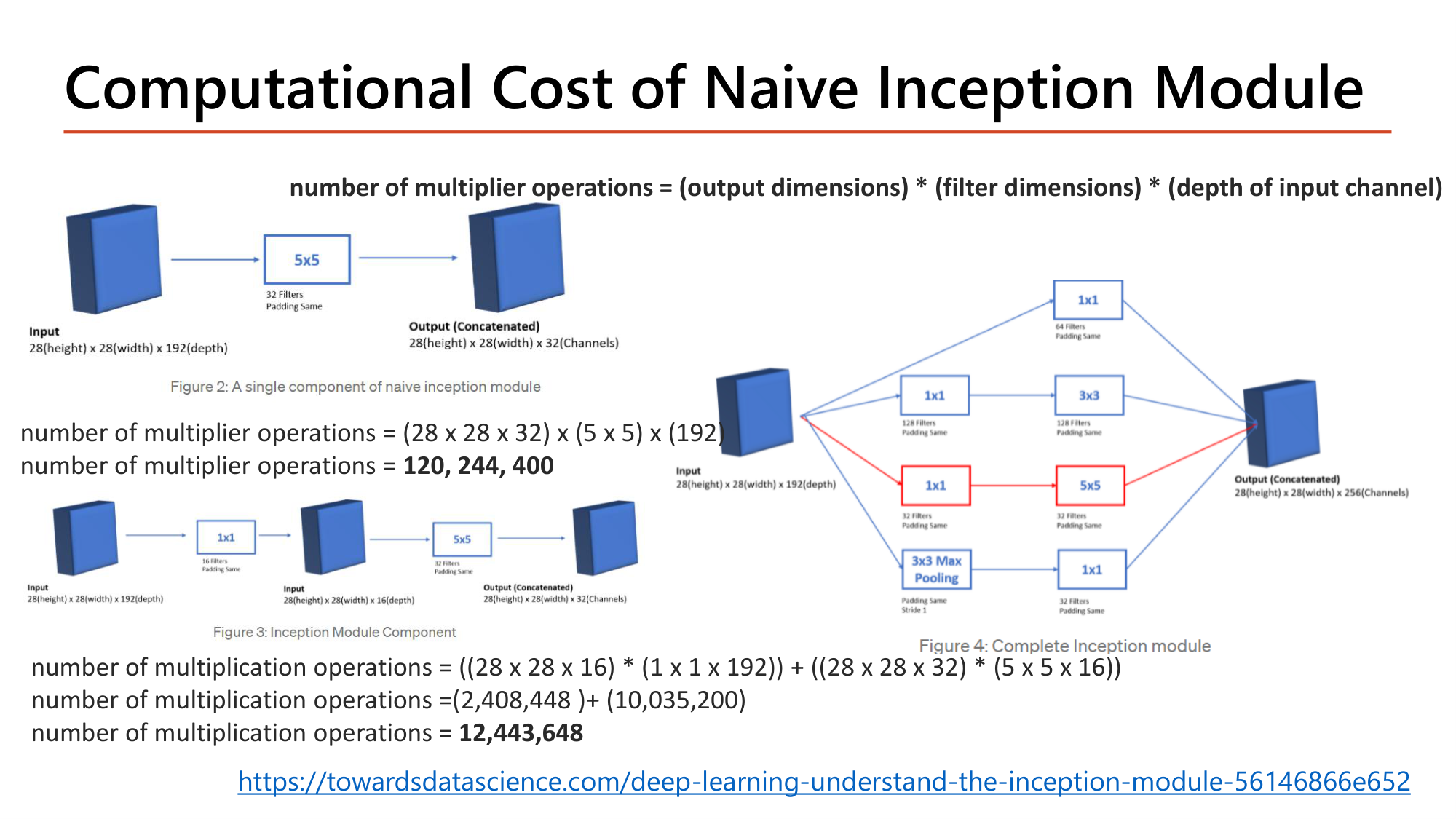
  1. input ถูก copy ส่งเข้า 4 เส้นทางขนาน: (ก) conv 1×1 (ข) conv 1×1 → conv 3×3 (ค) conv 1×1 → conv 5×5 (ง) max pool 3×3 → conv 1×1
  2. ทุก layer ใช้ stride 1 และ padding "same" จึงได้ output กว้าง×สูงเท่ากันทุกเส้นทาง
  3. conv 1×1 (เรียกว่า bottleneck layer) เรียน pattern ข้าม depth ของ input และลด depth ลง จึงลดการคำนวณ
  4. convolutional layer ทุกตัวใช้ ReLU
  5. ผลของ 4 เส้นทางถูก concatenate ตาม depth เป็นบล็อก Filter Concatenation
Slide: Computational Cost of Naive Inception Module. Number of multiplier operations = (output dimensions) * (filter dimensions) * (depth of input channel). Naive: input 28x28x192 through 5x5 conv with 32 filters gives (28x28x32) x (5x5) x 192. With a 1x1 conv of 16 filters first: ((28x28x16)*(1x1x192)) + ((28x28x32)*(5x5x16)) = 2,408,448 + 10,035,200 = 12,443,648
Slide: Computational Cost of Naive Inception Module (Lecture8, p.10)
$$\begin{gathered}\#\text{multiplications} = (\text{output dimensions})\\ \times\, (\text{filter dimensions}) \times (\text{depth of input channel})\end{gathered}$$

ทุกค่าของ output ต้องคูณ f×f ครั้งต่อ channel ของ input

คำนวณตามสไลด์: ต้นทุนของ conv 5×5 แบบตรง เทียบกับมี 1×1 bottleneck
ให้ input 28×28×192. ต้องการ output 28×28×32 จาก conv 5×5 (padding same)
  1. ขั้นที่ 1 — Naive: conv 5×5 จำนวน 32 filter บน 192 channel โดยตรง
    $$\begin{gathered}(28 \times 28 \times 32) \times (5 \times 5) \times 192\\ = 25{,}088 \times 25 \times 192 = 120{,}422{,}400\end{gathered}$$
  2. ขั้นที่ 2 — Bottleneck ส่วนแรก: conv 1×1 จำนวน 16 filter ลด depth จาก 192 เป็น 16
    $$\begin{gathered}(28 \times 28 \times 16) \times (1 \times 1) \times 192 \\[0.35em] = 12{,}544 \times 192 = 2{,}408{,}448\end{gathered}$$
  3. ขั้นที่ 3 — Bottleneck ส่วนที่สอง: conv 5×5 จำนวน 32 filter บน 16 channel
    $$\begin{gathered}(28 \times 28 \times 32) \times (5 \times 5) \times 16 \\[0.35em] = 25{,}088 \times 400 = 10{,}035{,}200\end{gathered}$$
  4. ขั้นที่ 4 — รวมและเทียบ
    $$\begin{gathered}2{,}408{,}448 + 10{,}035{,}200 = 12{,}443{,}648 \\[0.35em] \frac{120{,}422{,}400}{12{,}443{,}648} \approx 9.7\end{gathered}$$

Output เท่ากัน (28×28×32) แต่การคูณลดลงราว 9.7 เท่า. หมายเหตุ: สไลด์พิมพ์ผลของขั้นที่ 1 ว่า "120, 244, 400" ซึ่งสลับหลัก ค่าที่ถูกจากการคูณ 25,088 × 25 × 192 คือ 120,422,400. ค่า 2,408,448, 10,035,200 และ 12,443,648 ในสไลด์ถูกต้อง.
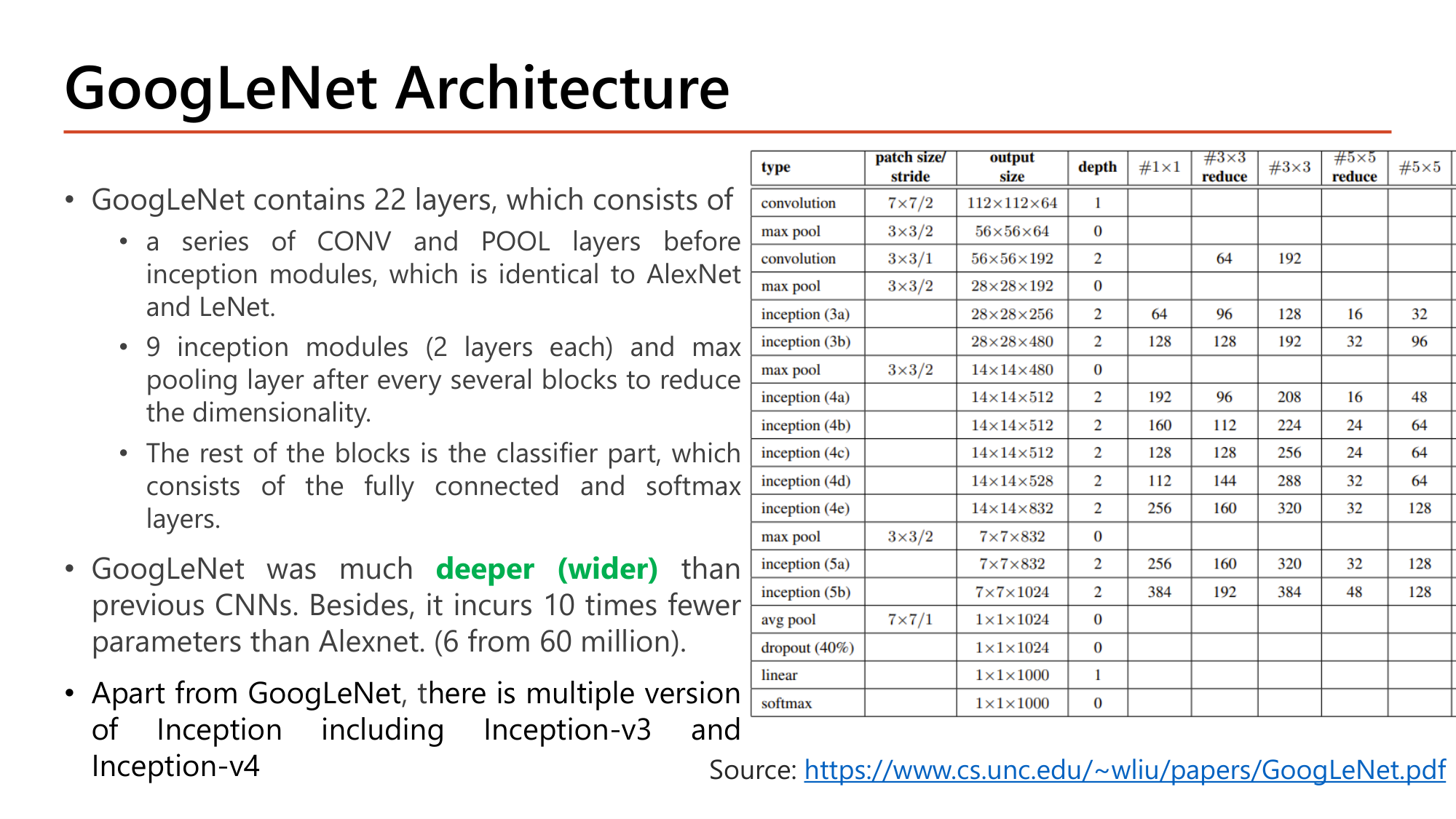
Slide: GoogLeNet Architecture contains 22 layers: a series of CONV and POOL layers before inception modules (identical to AlexNet and LeNet); 9 inception modules (2 layers each) with max pooling after every several blocks; the classifier part with fully connected and softmax layers. GoogLeNet was much deeper (wider) than previous CNNs and incurs 10 times fewer parameters than AlexNet (6 from 60 million). Table of layers: inception (3a) output 28x28x256 with 1x1=64, 3x3 reduce=96, 3x3=128, 5x5 reduce=16, 5x5=32, pool proj=32
Slide: GoogLeNet Architecture — 22 layers (Lecture8, p.11)

GoogLeNet มี 22 layers: (1) ชุด CONV และ POOL ก่อน inception module เหมือน AlexNet และ LeNet (2) inception module 9 ตัว (ตัวละ 2 layers) มี max pooling คั่นทุกสองสามบล็อกเพื่อลดมิติ (3) ส่วน classifier คือ fully connected และ softmax. GoogLeNet deeper (wider) กว่า CNN ก่อนหน้ามาก แต่ใช้ parameter น้อยกว่า AlexNet 10 เท่า (6 ล้าน จาก 60 ล้าน). Inception มีรุ่นอื่นอีก เช่น Inception-v3 และ Inception-v4.

คำนวณตามตารางในสไลด์: depth ของ output ของ inception (3a) และ (3b)
ให้ แถว inception (3a): #1×1 = 64, #3×3 reduce = 96, #3×3 = 128, #5×5 reduce = 16, #5×5 = 32, pool proj = 32. Input 28×28×192
  1. ขั้นที่ 1 — เลือก filter ที่เป็นปลายทางของแต่ละเส้นทาง (ค่า reduce เป็นขั้นกลาง ไม่ถูกนำมาต่อ)
    $$\text{1×1}: 64 \qquad \text{3×3}: 128 \qquad \text{5×5}: 32 \qquad \text{pool proj}: 32$$
  2. ขั้นที่ 2 — Concatenate ตาม depth = บวกจำนวน channel
    $$64 + 128 + 32 + 32 = 256 \quad\Rightarrow\quad 28 \times 28 \times 256$$
  3. ขั้นที่ 3 — inception (3b): 128, 192, 96, 64
    $$128 + 192 + 96 + 64 = 480 \quad\Rightarrow\quad 28 \times 28 \times 480$$

256 และ 480 ตรงกับคอลัมน์ output size ของตาราง. กว้างและสูงคงเดิม (28×28) เพราะทุกเส้นทางใช้ padding same; การ concatenate เปลี่ยนเฉพาะ depth.
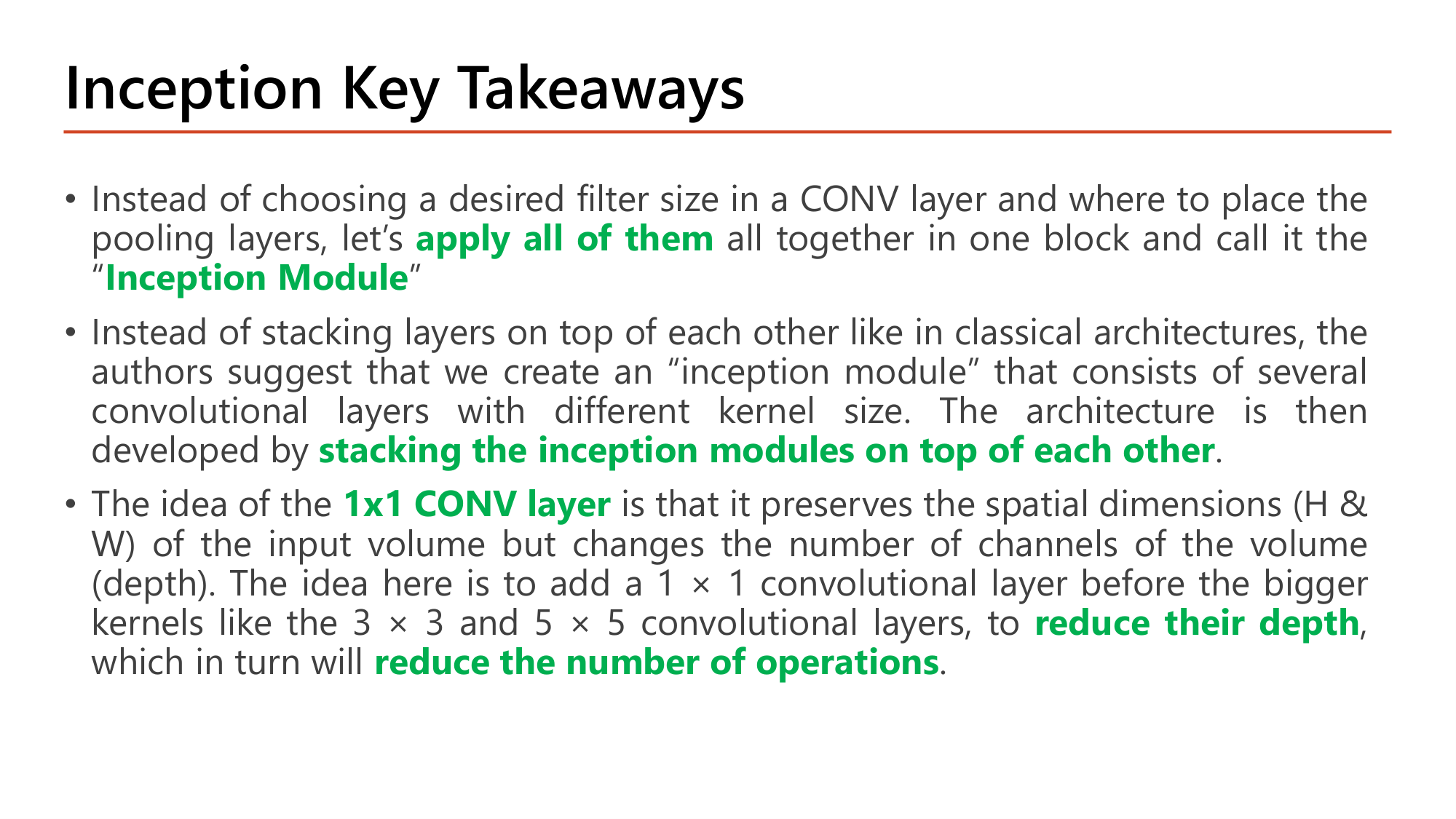
Slide: Inception Key Takeaways. Instead of choosing a desired filter size in a CONV layer and where to place the pooling layers, apply all of them together in one block called the Inception Module. The architecture is developed by stacking the inception modules on top of each other. The 1x1 CONV layer preserves spatial dimensions (H and W) but changes the number of channels (depth); adding a 1x1 conv before bigger 3x3 and 5x5 kernels reduces their depth, which reduces the number of operations
Slide: Inception Key Takeaways (Lecture8, p.12)
คำถาม 6Inception
Inception module หนึ่งรับ input 14×14×480 เส้นทางทั้งสี่ให้ output 192, 208, 48 และ 64 channel ตามลำดับ (ทุกเส้นทาง stride 1 padding same) shape หลัง depth concatenation คือข้อใด?
คำถาม 7Inception
Input 14×14×256 ต้องการ output 14×14×64 จาก conv 5×5 (padding same) ถ้าใส่ conv 1×1 จำนวน 32 filter ไว้ก่อน จำนวนการคูณทั้งหมดคือเท่าใด เมื่อใช้สูตร (ขนาด output) × (ขนาด filter) × (depth ของ input)?
ออกสอบสูง — ข้อความที่อาจารย์ทำสี

6. ResNet (2015): skip connection ทำให้ network ลึกมากเทรนได้

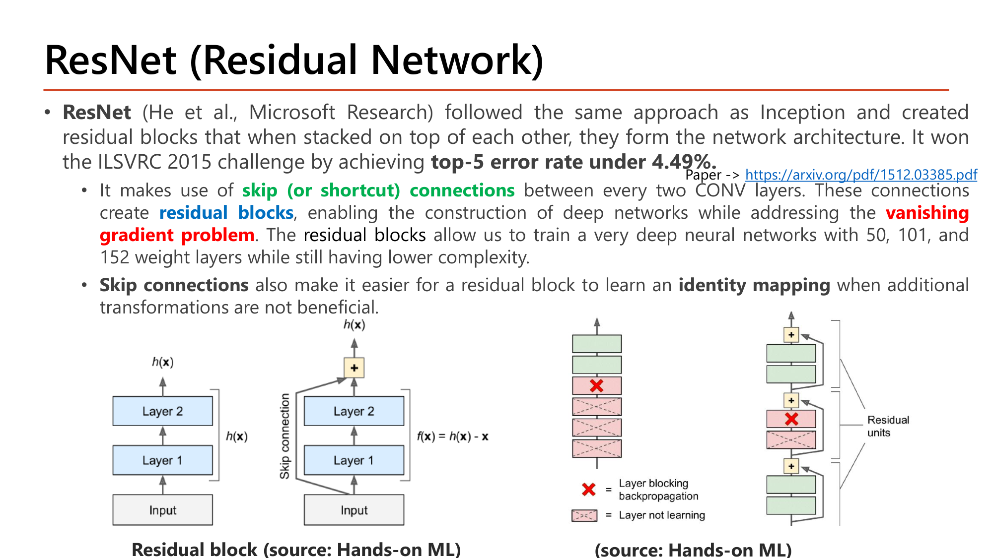
Slide: ResNet (He et al., Microsoft Research) created residual blocks stacked to form the network; won ILSVRC 2015 with top-5 error 4.49%. Uses skip (shortcut) connections between every two CONV layers, creating residual blocks that address the vanishing gradient problem and allow training networks with 50, 101 and 152 weight layers. Skip connections make it easier to learn an identity mapping. Diagram: plain block outputs h(x); residual block has f(x) = h(x) - x with a skip connection added back; when a layer blocks backpropagation the signal still flows through the skip
Slide: ResNet (Residual Network) — residual block (Lecture8, p.13)

ResNet (He et al., Microsoft Research) ใช้แนวทางเดียวกับ Inception คือสร้างบล็อกแล้วนำมาซ้อน. ชนะ ILSVRC 2015 ด้วย top-5 error rate 4.49%. ใช้ skip (or shortcut) connections ระหว่างทุกสอง CONV layer. การเชื่อมนี้สร้าง residual blocks ซึ่งทำให้สร้าง network ลึกได้โดยแก้ vanishing gradient problem. จึงเทรน network ที่มี 50, 101 และ 152 weight layers ได้โดยยังมี complexity ต่ำกว่า. Skip connection ยังทำให้ residual block เรียน identity mapping ได้ง่ายเมื่อการแปลงเพิ่มเติมไม่มีประโยชน์.

ต้องรู้ก่อน — ทำไม network ลึกจึงเทรนยาก

Backpropagation คูณ gradient ย้อนกลับทีละ layer (Lesson 3). ถ้าตัวคูณแต่ละชั้นเล็กกว่า 1 ผลคูณหลายสิบชั้นจะเข้าใกล้ศูนย์ layer ต้นๆ จึงแทบไม่ถูกอัปเดต (Lesson 5). เช่น \(0.8^{50} \approx 0.000014\).

รูปซ้ายของสไลด์เทียบสองบล็อก. ให้ \(h(x)\) คือฟังก์ชันที่ต้องการให้บล็อกเรียน.

$$h(x) = f(x) + x \qquad\Longleftrightarrow\qquad f(x) = h(x) - x$$

บล็อกเรียนเฉพาะ "ส่วนที่ต้องเพิ่มจาก input" (residual) ไม่ต้องสร้าง output ทั้งหมดใหม่

คำนวณ: identity mapping และ gradient ผ่าน skip connection
ให้ residual block มี output \(h(x) = f(x) + x\)
  1. ขั้นที่ 1 — ถ้า weight ของสอง layer เป็นศูนย์ทั้งหมด
    $$f(x) = 0 \quad\Rightarrow\quad h(x) = 0 + x = x$$

    บล็อกกลายเป็น identity โดยไม่ต้องเรียนอะไร. บล็อกธรรมดาที่ weight เป็นศูนย์ให้ output 0 และตัดสัญญาณทิ้ง

  2. ขั้นที่ 2 — Gradient ของ output เทียบกับ input
    $$\frac{\partial h}{\partial x} = \frac{\partial f}{\partial x} + 1$$
  3. ขั้นที่ 3 — ถ้า \(\partial f / \partial x = 0.01\) (layer เกือบปิดกั้น gradient)
    $$\text{บล็อกธรรมดา: } 0.01 \qquad \text{residual block: } 0.01 + 1 = 1.01$$

พจน์ "+1" คือเส้นทางลัดที่ gradient ไหลย้อนกลับได้โดยไม่ถูกคูณด้วยค่าเล็ก. รูปขวาของสไลด์แสดงกรณีนี้: layer ที่มีกากบาท (blocking backpropagation) ไม่ทำให้ layer ก่อนหน้าหยุดเรียน เพราะสัญญาณอ้อมผ่าน skip connection.
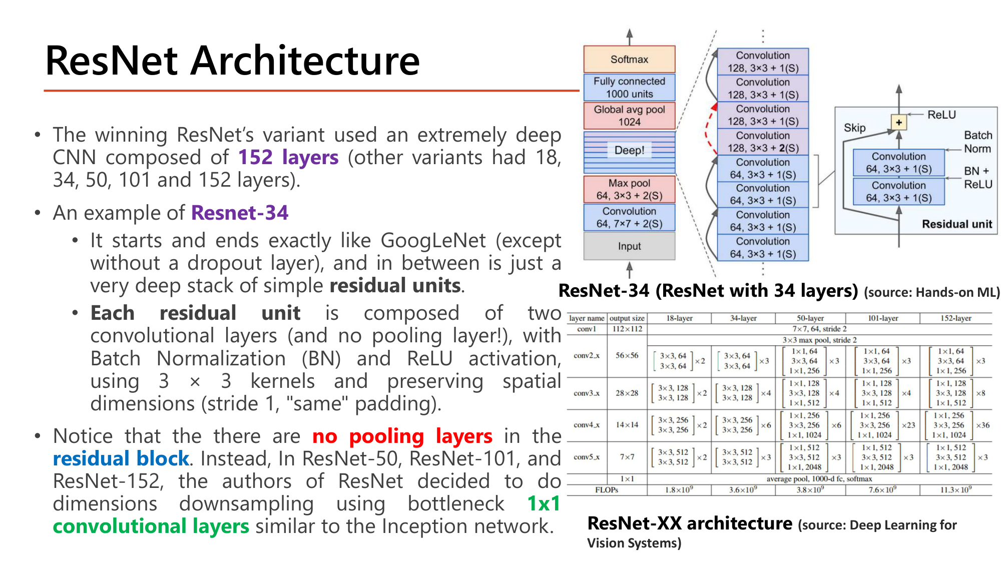
Slide: ResNet Architecture. The winning variant used 152 layers (variants 18, 34, 50, 101, 152). ResNet-34 starts and ends like GoogLeNet (without dropout) with a deep stack of residual units in between. Each residual unit has two convolutional layers (no pooling layer), with Batch Normalization and ReLU, 3x3 kernels, stride 1, same padding. No pooling layers in the residual block; ResNet-50/101/152 use bottleneck 1x1 convolutional layers. Table of ResNet-18/34/50/101/152 block counts and FLOPs
Slide: ResNet Architecture — ResNet-34 และตารางรุ่นต่างๆ (Lecture8, p.14)

รุ่นที่ชนะใช้ CNN ลึก 152 layers (รุ่นอื่นมี 18, 34, 50, 101). ตัวอย่างในสไลด์คือ Resnet-34:

คำนวณตามตารางในสไลด์: นับ layer ของ ResNet-34 และ ResNet-50
ให้ ทั้งสองรุ่นมีจำนวนบล็อกต่อ stage (conv2_x ถึง conv5_x) = 3, 4, 6, 3. ResNet-34 ใช้บล็อก 2 conv; ResNet-50 ใช้ bottleneck 3 conv (1×1, 3×3, 1×1)
  1. ขั้นที่ 1 — ResNet-34
    $$\underbrace{1}_{\text{conv1}} + \underbrace{(3 + 4 + 6 + 3) \times 2}_{32} + \underbrace{1}_{\text{FC}} = 34$$
  2. ขั้นที่ 2 — ResNet-50
    $$1 + (3 + 4 + 6 + 3) \times 3 + 1 = 1 + 48 + 1 = 50$$
  3. ขั้นที่ 3 — ResNet-152: บล็อกต่อ stage = 3, 8, 36, 3 (bottleneck)
    $$1 + (3 + 8 + 36 + 3) \times 3 + 1 = 1 + 150 + 1 = 152$$

ตัวเลขในชื่อรุ่นคือจำนวน weight layers. Pooling และ BN ไม่นับ.
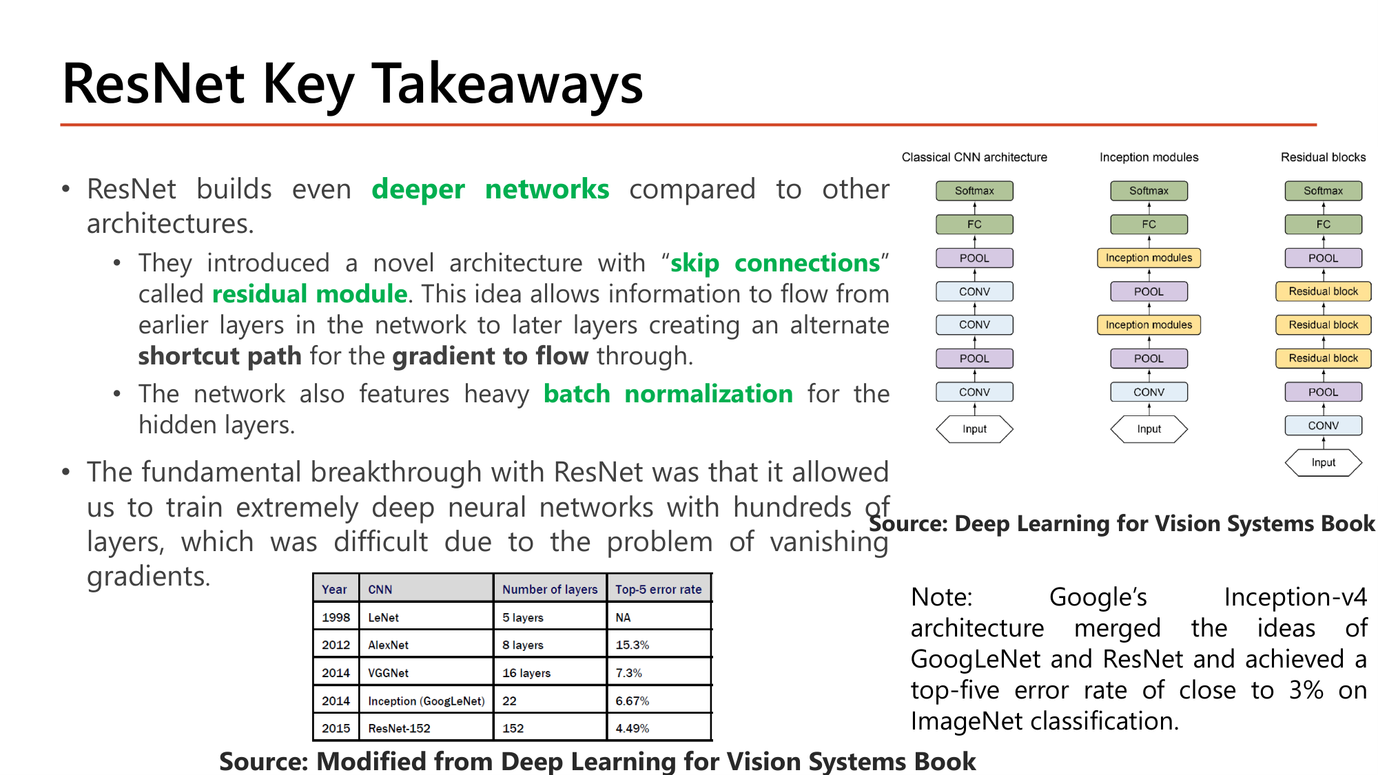
Slide: ResNet Key Takeaways. ResNet builds even deeper networks; skip connections called residual module allow information to flow from earlier to later layers, creating an alternate shortcut path for the gradient; heavy batch normalization for the hidden layers. The breakthrough: training extremely deep networks with hundreds of layers. Table: 1998 LeNet 5 layers; 2012 AlexNet 8 layers 15.3%; 2014 VGGNet 16 layers 7.3%; 2014 Inception (GoogLeNet) 22 layers 6.67%; 2015 ResNet-152 152 layers 4.49%. Note: Inception-v4 merged GoogLeNet and ResNet, top-five error close to 3%
Slide: ResNet Key Takeaways — ตารางสรุป 5 รุ่น (Lecture8, p.15)
YearCNNNumber of layersTop-5 error rate
1998LeNet5 layersNA
2012AlexNet8 layers15.3%
2014VGGNet16 layers7.3%
2014Inception (GoogLeNet)226.67%
2015ResNet-1521524.49%

จำนวน layer เพิ่มทุกรุ่น (5 → 8 → 16 → 22 → 152) และ error ลดทุกรุ่น (15.3 → 7.3 → 6.67 → 4.49). หมายเหตุในสไลด์: Inception-v4 ของ Google รวมแนวคิดของ GoogLeNet และ ResNet ได้ top-five error ใกล้ 3%.
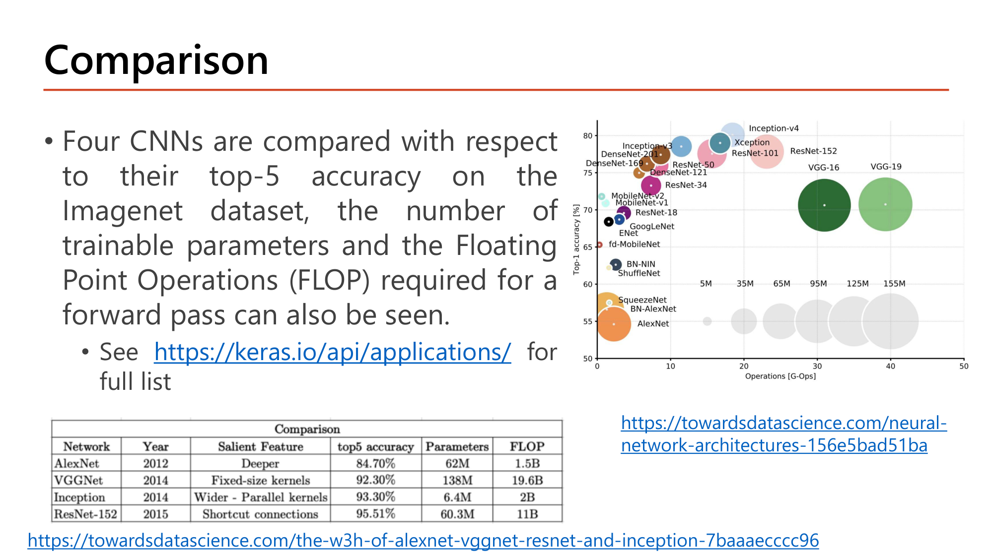
Slide: Comparison. Four CNNs compared on top-5 accuracy, trainable parameters and FLOPs. AlexNet 2012 Deeper 84.70% 62M 1.5B. VGGNet 2014 Fixed-size kernels 92.30% 138M 19.6B. Inception 2014 Wider, Parallel kernels 93.30% 6.4M 2B. ResNet-152 2015 Shortcut connections 95.51% 60.3M 11B. Bubble chart of top-1 accuracy versus operations
Slide: Comparison — accuracy, parameters, FLOP (Lecture8, p.16)
NetworkYearSalient Featuretop5 accuracyParametersFLOP
AlexNet2012Deeper84.70%62M1.5B
VGGNet2014Fixed-size kernels92.30%138M19.6B
Inception2014Wider - Parallel kernels93.30%6.4M2B
ResNet-1522015Shortcut connections95.51%60.3M11B

FLOP (Floating Point Operations) คือจำนวนการคำนวณของ forward pass หนึ่งครั้ง. อ่านตารางเป็นการแลกเปลี่ยน: Inception ได้ accuracy สูงกว่า VGGNet 1 จุด (93.30 เทียบกับ 92.30) ด้วย parameter น้อยกว่า \(138 / 6.4 \approx 21.6\) เท่า และ FLOP น้อยกว่า \(19.6 / 2 \approx 9.8\) เท่า. ResNet-152 ลึกกว่า VGG16 เกือบ 10 เท่า (152 เทียบกับ 16 layers) แต่มี parameter น้อยกว่าครึ่ง (60.3M เทียบกับ 138M). ความสัมพันธ์ accuracy กับ error: \(100 - 95.51 = 4.49\%\) ตรงกับ top-5 error ของ ResNet-152.
คำถาม 8ResNet
ใน residual block ถ้า h(x) คือ output ของทั้งบล็อกและ x คือ input สอง convolutional layer ภายในบล็อกเรียนฟังก์ชัน f(x) ที่สัมพันธ์กับ h(x) อย่างไร?
คำถาม 9ResNet
ResNet รุ่นหนึ่งมี convolution แรก 1 ชั้น ตามด้วย residual unit แบบ 2 convolution จำนวน 2, 2, 2, 2 ตัวในสี่ stage และ fully connected 1 ชั้น network นี้มีกี่ weight layers?
คำถาม 10Comparison
ข้อใดจับคู่สถาปัตยกรรมกับจุดเด่น (salient feature) ได้ถูกต้องทั้งหมด?
ออกสอบสูง — ข้อความที่อาจารย์ทำสี

7. Modern CNNs และหลักออกแบบสถาปัตยกรรม

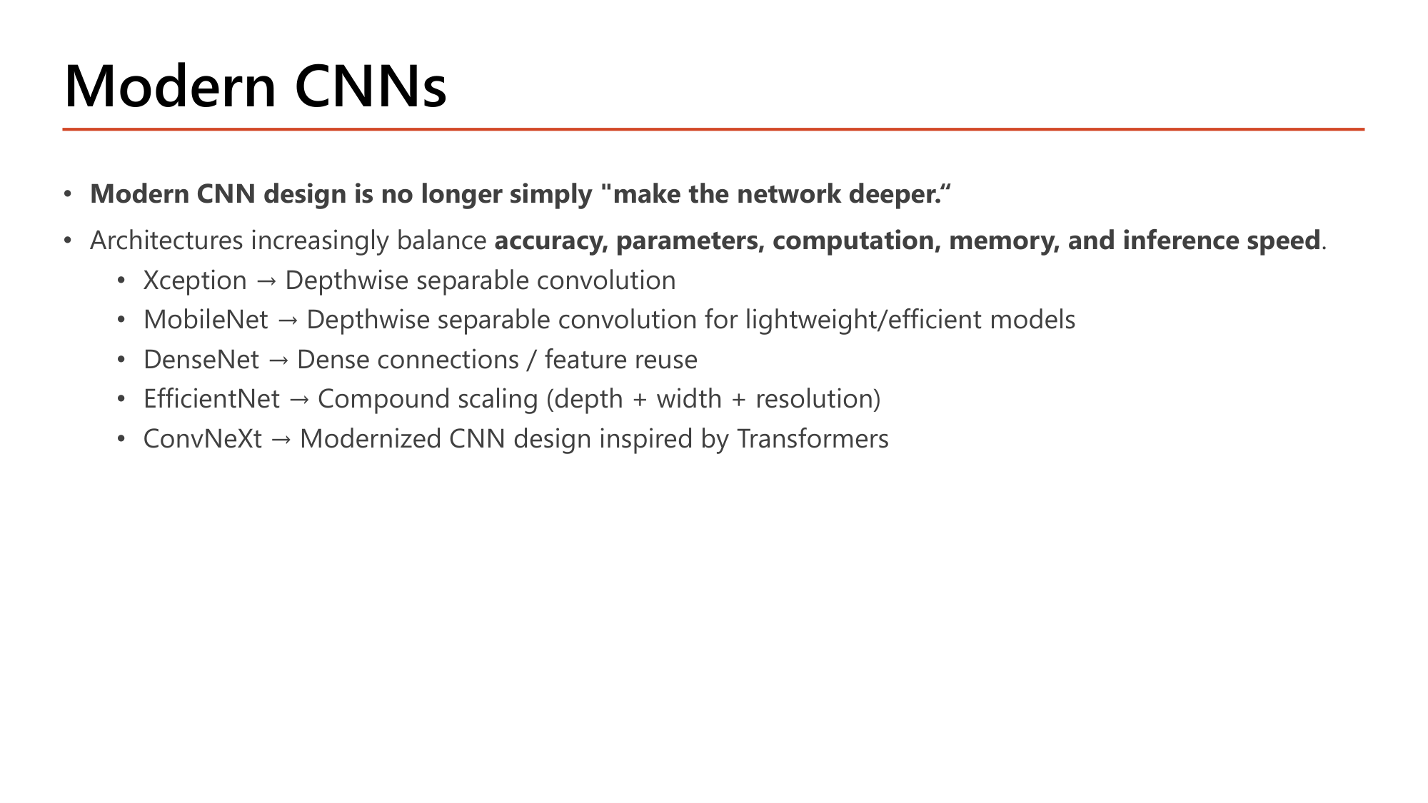
Slide: Modern CNNs. Modern CNN design is no longer simply make the network deeper. Architectures increasingly balance accuracy, parameters, computation, memory, and inference speed. Xception: depthwise separable convolution. MobileNet: depthwise separable convolution for lightweight/efficient models. DenseNet: dense connections / feature reuse. EfficientNet: compound scaling (depth + width + resolution). ConvNeXt: modernized CNN design inspired by Transformers
Slide: Modern CNNs — ไม่ใช่แค่ลึกขึ้น (Lecture8, p.17)

Modern CNN design is no longer simply "make the network deeper." สถาปัตยกรรมรุ่นใหม่ต้องสมดุล accuracy, parameters, computation, memory, and inference speed. ห้ารุ่นและแนวคิดหลัก:

รุ่นแนวคิดหลัก
XceptionDepthwise separable convolution
MobileNetDepthwise separable convolution for lightweight/efficient models
DenseNetDense connections / feature reuse
EfficientNetCompound scaling (depth + width + resolution)
ConvNeXtModernized CNN design inspired by Transformers
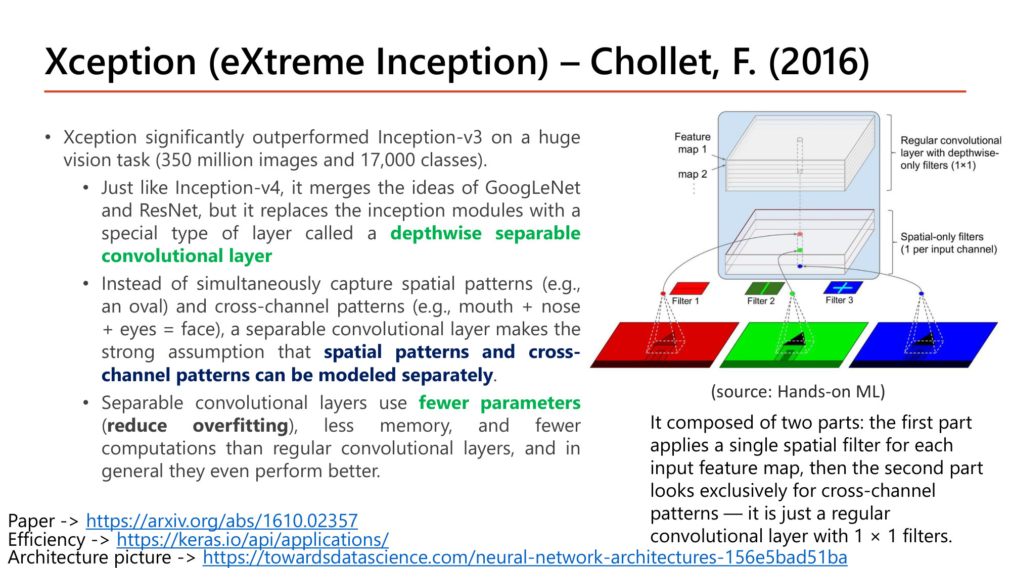
Slide: Xception (eXtreme Inception), Chollet 2016. Outperformed Inception-v3 on a huge vision task (350 million images, 17,000 classes). Merges ideas of GoogLeNet and ResNet but replaces inception modules with depthwise separable convolutional layers, assuming spatial patterns and cross-channel patterns can be modeled separately. Uses fewer parameters, less memory, fewer computations. Diagram: spatial-only filters (1 per input channel) followed by a regular convolutional layer with 1x1 filters
Slide: Xception — depthwise separable convolution (Lecture8, p.18)

Xception (eXtreme Inception; Chollet, 2016) ทำได้ดีกว่า Inception-v3 อย่างชัดเจนในงานขนาดใหญ่ (350 ล้านภาพ, 17,000 class). เหมือน Inception-v4 ตรงที่รวมแนวคิดของ GoogLeNet และ ResNet แต่แทน inception module ด้วย depthwise separable convolutional layer.

Convolution ปกติจับ spatial pattern (เช่น รูปวงรี) และ cross-channel pattern (เช่น ปาก + จมูก + ตา = หน้า) พร้อมกัน. Separable convolution ตั้งสมมติฐานว่า spatial patterns and cross- channel patterns can be modeled separately จึงแบ่งเป็นสองส่วน:

  1. Depthwise (spatial-only filters): ใช้ spatial filter 1 ตัวต่อ 1 input feature map (1 per input channel)
  2. Pointwise: convolutional layer ปกติที่ใช้ filter 1×1 ซึ่งมองหาเฉพาะ cross-channel pattern

Separable convolutional layer ใช้ fewer parameters (reduce overfitting) ใช้ memory น้อยกว่า และคำนวณน้อยกว่า convolution ปกติ และโดยทั่วไปทำงานได้ดีกว่าด้วย.

คำนวณ: parameter ของ convolution ปกติเทียบกับ depthwise separable
ให้ kernel 3×3, input 64 channel, output 128 channel
  1. ขั้นที่ 1 — Convolution ปกติ
    $$(3 \cdot 3 \cdot 64 + 1) \cdot 128 = 73{,}856$$
  2. ขั้นที่ 2 — Depthwise: filter 3×3 หนึ่งตัวต่อ input channel
    $$3 \cdot 3 \cdot 64 = 576$$
  3. ขั้นที่ 3 — Pointwise: conv 1×1 จาก 64 เป็น 128 channel พร้อม bias
    $$1 \cdot 1 \cdot 64 \cdot 128 + 128 = 8{,}320$$
  4. ขั้นที่ 4 — รวมและเทียบ
    $$576 + 8{,}320 = 8{,}896 \qquad \frac{73{,}856}{8{,}896} \approx 8.3$$

Separable convolution ใช้ parameter น้อยกว่าราว 8.3 เท่าสำหรับ output shape เดียวกัน. ค่า 8,896 คือค่าที่ SeparableConv2D(128, 3) ของ Keras รายงานเมื่อ input มี 64 channel.
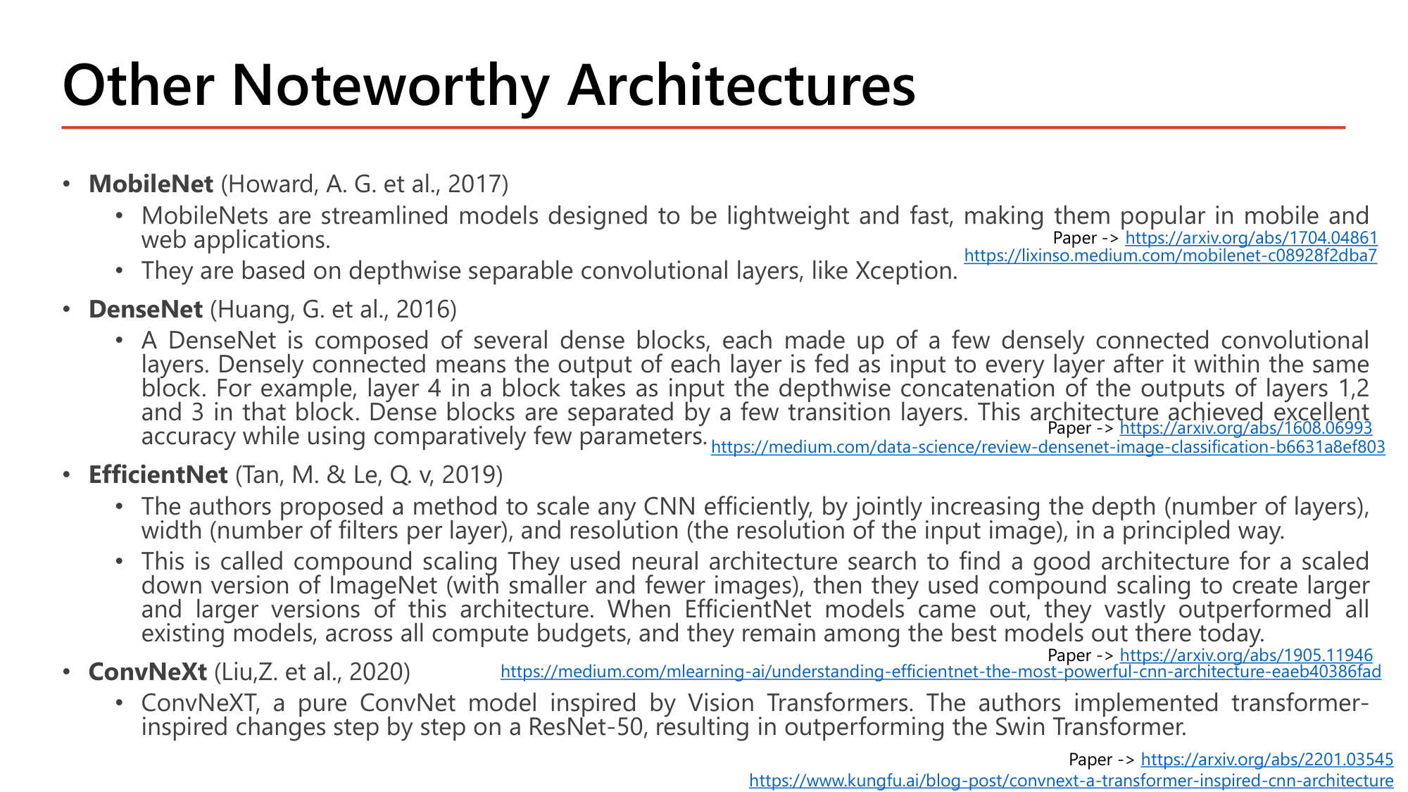
Slide: Other Noteworthy Architectures. MobileNet (2017): streamlined, lightweight and fast models for mobile and web, based on depthwise separable convolutional layers. DenseNet (2016): dense blocks where the output of each layer is fed as input to every layer after it within the same block; layer 4 takes the depthwise concatenation of outputs of layers 1, 2 and 3; few parameters. EfficientNet (2019): compound scaling of depth, width and resolution; neural architecture search. ConvNeXt: pure ConvNet inspired by Vision Transformers, built step by step on ResNet-50, outperforming Swin Transformer
Slide: Other Noteworthy Architectures (Lecture8, p.19)
รุ่นสาระสำคัญตามสไลด์
MobileNet (Howard et al., 2017)โมเดลที่ออกแบบให้ lightweight และ fast นิยมใช้ใน mobile และ web application. ใช้ depthwise separable convolutional layer เหมือน Xception
DenseNet (Huang et al., 2016)ประกอบด้วย dense block หลายตัว. Densely connected หมายถึง output ของแต่ละ layer ถูกป้อนเป็น input ให้ทุก layer ถัดไปใน block เดียวกัน. เช่น layer 4 รับ depthwise concatenation ของ output จาก layer 1, 2 และ 3. Dense block คั่นด้วย transition layer. ได้ accuracy ดีมากด้วย parameter ค่อนข้างน้อย
EfficientNet (Tan & Le, 2019)วิธี scale CNN อย่างมีหลักการโดยเพิ่ม depth (จำนวน layer), width (จำนวน filter ต่อ layer) และ resolution (ความละเอียดของภาพ input) ร่วมกัน เรียกว่า compound scaling. ใช้ neural architecture search หาสถาปัตยกรรมตั้งต้นบน ImageNet ฉบับย่อ แล้ว scale ขึ้น
ConvNeXt (Liu et al.)ConvNet ล้วนที่ได้แรงบันดาลใจจาก Vision Transformer. ปรับ ResNet-50 ทีละขั้นด้วยแนวคิดจาก transformer จนทำได้ดีกว่า Swin Transformer

ตัวอย่าง DenseNet เป็นตัวเลข: ถ้าทุก layer ใน block ให้ output 32 channel และ input ของ block มี 64 channel, layer 4 จะรับ \(64 + 32 + 32 + 32 = 160\) channel. การนำ feature เดิมกลับมาใช้ (feature reuse) ทำให้แต่ละ layer ต้องผลิต feature ใหม่เพียงเล็กน้อย.
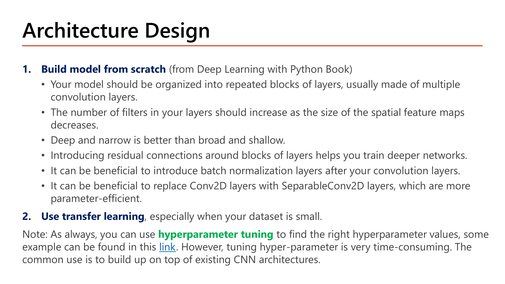
Slide: Architecture Design. 1. Build model from scratch: organize into repeated blocks of layers; number of filters should increase as spatial feature maps decrease; deep and narrow is better than broad and shallow; residual connections help train deeper networks; batch normalization after convolution layers can be beneficial; replace Conv2D with SeparableConv2D for parameter efficiency. 2. Use transfer learning, especially when your dataset is small. Note: hyperparameter tuning is very time-consuming; the common use is to build on top of existing CNN architectures
Slide: Architecture Design — สองทางเลือก (Lecture8, p.20)

เมื่อต้องสร้าง CNN มีสองทางเลือก.

1. Build model from scratch (หลักจากหนังสือ Deep Learning with Python):

2. Use transfer learning โดยเฉพาะเมื่อ dataset เล็ก.

หมายเหตุ: ใช้ hyperparameter tuning (Lesson 6) หาค่าที่เหมาะได้ แต่ใช้เวลามาก. วิธีที่ใช้ทั่วไปคือสร้างต่อยอดจากสถาปัตยกรรม CNN ที่มีอยู่.
คำถาม 11Separable convolution
Depthwise separable convolution ใช้ kernel 3×3 กับ input 32 channel และให้ output 64 channel ถ้าไม่นับ bias layer นี้มี weight กี่ตัว?
คำถาม 12Modern CNN
ข้อใดอธิบาย compound scaling ของ EfficientNet ได้ถูกต้อง?
ออกสอบสูง — ข้อความที่อาจารย์ทำสี

8. Transfer Learning: แนวคิด สามแนวทาง และ Guidelines

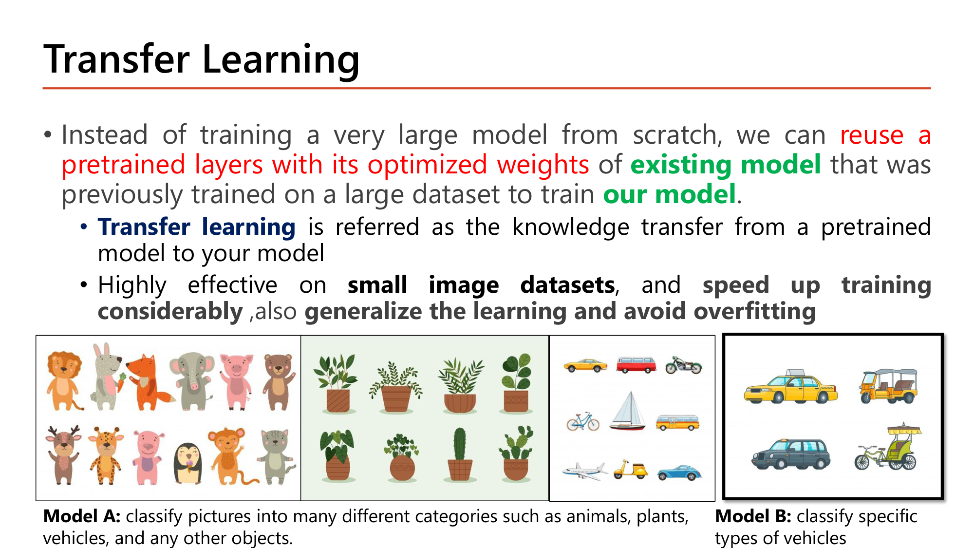
Slide: Transfer Learning. Instead of training a very large model from scratch, we can reuse pretrained layers with their optimized weights of an existing model previously trained on a large dataset to train our model. Transfer learning is knowledge transfer from a pretrained model to your model. Highly effective on small image datasets, speeds up training considerably, generalizes the learning and avoids overfitting. Model A classifies pictures into many categories (animals, plants, vehicles); Model B classifies specific types of vehicles
Slide: Transfer Learning — Model A และ Model B (Lecture8, p.21)

แทนการเทรนโมเดลขนาดใหญ่มากจากศูนย์ เราสามารถ reuse a pretrained layers with its optimized weights ของ existing model ที่เทรนบน dataset ขนาดใหญ่มาแล้ว เพื่อเทรน our model. Transfer learning คือการถ่ายโอนความรู้จาก pretrained model มายังโมเดลของเรา. ได้ผลดีมากกับ small image datasets, speed up training considerably และ generalize the learning and avoid overfitting.

ตัวอย่างในสไลด์: Model A จำแนกภาพเป็นหลายประเภท (สัตว์, พืช, ยานพาหนะ และวัตถุอื่น). Model B ต้องจำแนกเฉพาะชนิดของยานพาหนะ (แท็กซี่, ตุ๊กตุ๊ก, รถตู้, สามล้อ). Model A เรียน feature ระดับล่าง (ขอบ, สี, ล้อ, กระจก) มาแล้ว Model B จึงนำ layer เหล่านั้นมาใช้ได้โดยไม่ต้องเรียนใหม่.
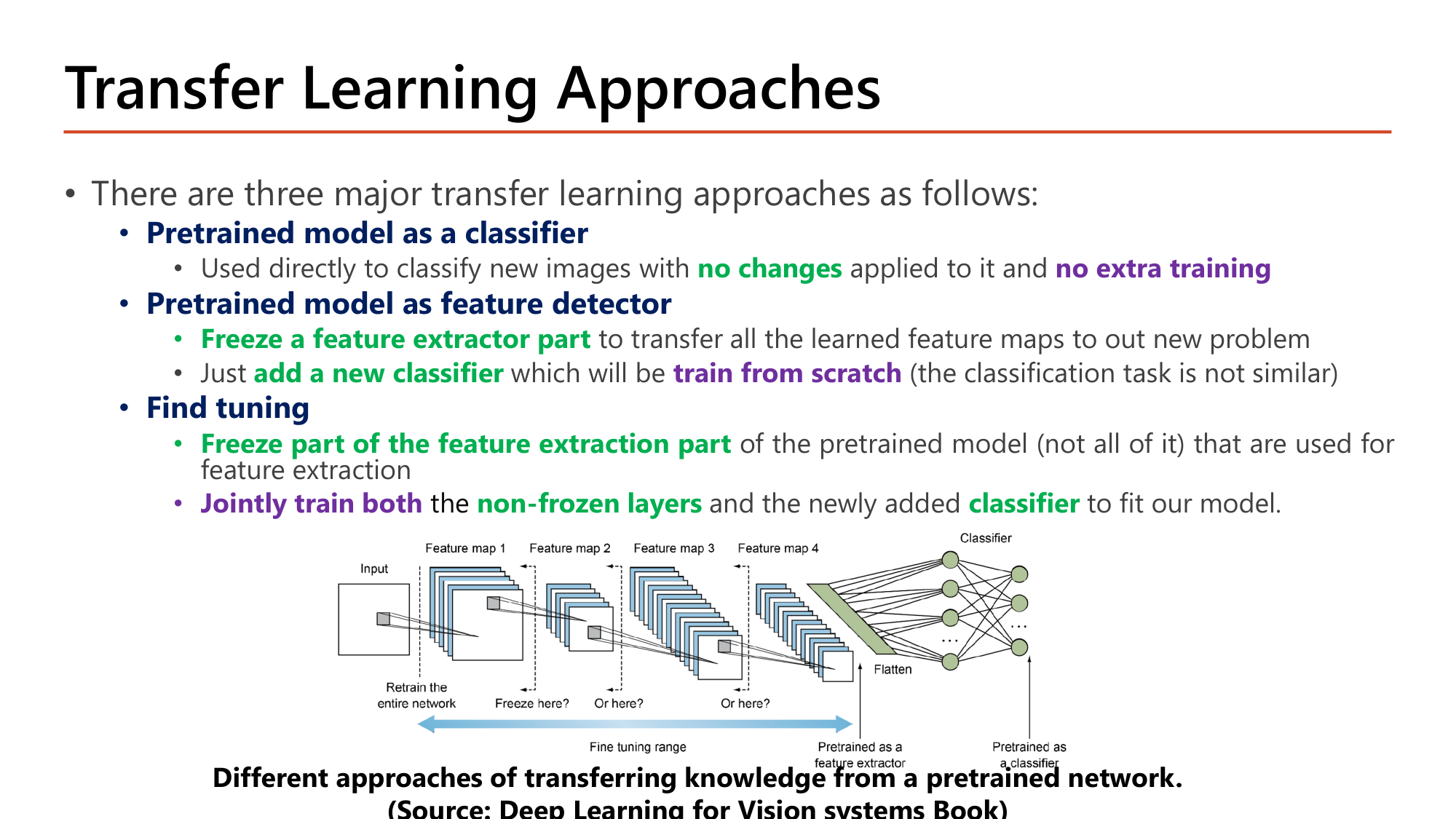
Slide: Transfer Learning Approaches. Three major approaches: (1) Pretrained model as a classifier: used directly with no changes and no extra training. (2) Pretrained model as feature detector: freeze the feature extractor part, add a new classifier trained from scratch. (3) Fine tuning: freeze part of the feature extraction part (not all), jointly train the non-frozen layers and the newly added classifier. Diagram shows freeze points along the network
Slide: Transfer Learning Approaches — สามแนวทาง (Lecture8, p.22)
แนวทางข้อความในสไลด์ส่วนที่ถูกเทรน
Pretrained model as a classifierใช้จำแนกภาพใหม่โดยตรง มี no changes และ no extra trainingไม่มี
Pretrained model as feature detectorFreeze a feature extractor part เพื่อถ่ายโอน feature map ที่เรียนแล้วทั้งหมด แล้ว add a new classifier ซึ่งจะ train from scratch (งานจำแนกไม่เหมือนเดิม)classifier ใหม่เท่านั้น
Find tuning (fine tuning)Freeze part of the feature extraction part ของ pretrained model (ไม่ใช่ทั้งหมด) แล้ว Jointly train both non-frozen layers และ classifier ที่เพิ่มใหม่layer ท้ายของ feature extractor + classifier ใหม่
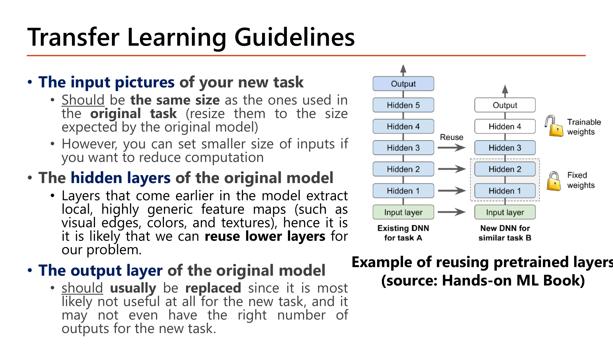
Slide: Transfer Learning Guidelines. Input pictures should be the same size as the original task (resize), but smaller inputs reduce computation. Hidden layers: earlier layers extract local, highly generic feature maps (edges, colors, textures), so lower layers can be reused. The output layer should usually be replaced: not useful for the new task and may not have the right number of outputs. Diagram: existing DNN for task A with hidden 1-5; new DNN for similar task B reuses hidden 1-4, hidden 1-2 fixed weights, hidden 3-4 trainable, new output
Slide: Transfer Learning Guidelines — input, hidden, output (Lecture8, p.23)

รูปในสไลด์: DNN เดิมของ task A มี Hidden 1–5. DNN ใหม่ของ task B ที่คล้ายกันนำ Hidden 1–4 มาใช้ โดย Hidden 1–2 เป็น fixed weights (frozen) และ Hidden 3–4 เป็น trainable weights. Hidden 5 และ Output เดิมถูกทิ้ง แล้วใส่ Output ใหม่.
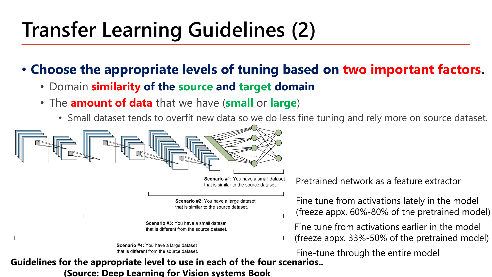
Slide: Transfer Learning Guidelines (2). Choose the appropriate level of tuning based on two factors: domain similarity of source and target domain, and the amount of data (small or large). Small dataset tends to overfit so do less fine tuning. Scenario 1 small and similar: pretrained network as feature extractor. Scenario 2 large and similar: fine tune from activations lately in the model (freeze 60-80%). Scenario 3 small and different: fine tune from activations earlier (freeze 33-50%). Scenario 4 large and different: fine-tune through the entire model
Slide: Transfer Learning Guidelines (2) — สี่สถานการณ์ (Lecture8, p.24)

Choose the appropriate levels of tuning based on two important factors. ได้แก่ (1) domain similarity of the source and target domain และ (2) amount of data ที่มี (small หรือ large). Dataset เล็กมักทำให้ overfit จึง fine tune น้อยลงและพึ่ง source dataset มากขึ้น.

Scenarioขนาด datasetความคล้ายกับ sourceระดับที่แนะนำ
#1smallsimilarPretrained network as a feature extractor
#2largesimilarFine tune from activations lately in the model (freeze ประมาณ 60%–80% ของ pretrained model)
#3smalldifferentFine tune from activations earlier in the model (freeze ประมาณ 33%–50%)
#4largedifferentFine-tune through the entire model

หลักเบื้องหลังตาราง: ยิ่ง domain ต่างจาก source มาก feature ระดับสูงของโมเดลเดิมยิ่งใช้ไม่ได้ จึงต้องปลด freeze ย้อนไปถึง layer ต้นขึ้น (freeze น้อยลง). ยิ่งข้อมูลมาก ยิ่งเทรน layer จำนวนมากได้โดยไม่ overfit.
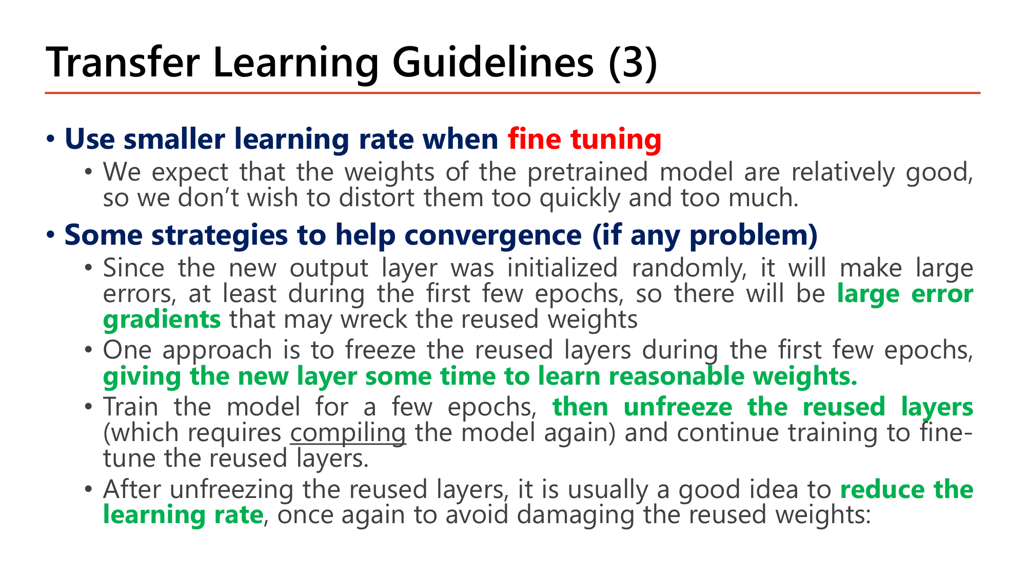
Slide: Transfer Learning Guidelines (3). Use smaller learning rate when fine tuning: pretrained weights are relatively good, do not distort them too quickly. Strategies to help convergence: the new output layer is initialized randomly so there will be large error gradients that may wreck the reused weights; freeze the reused layers during the first few epochs, giving the new layer time to learn reasonable weights; then unfreeze the reused layers (requires compiling the model again) and continue training; after unfreezing reduce the learning rate
Slide: Transfer Learning Guidelines (3) — learning rate และลำดับการเทรน (Lecture8, p.25)

Use smaller learning rate when fine tuning. weight ของ pretrained model ถือว่าดีอยู่แล้ว จึงไม่ต้องการบิดมันเร็วเกินและมากเกิน.

Some strategies to help convergence (if any problem):

  1. output layer ใหม่ถูกกำหนดค่าเริ่มต้นแบบสุ่ม จึงผิดพลาดมากในช่วง epoch แรกๆ ทำให้เกิด large error gradients ที่อาจทำลาย weight ที่นำมาใช้ซ้ำ
  2. วิธีหนึ่งคือ freeze layer ที่นำมาใช้ซ้ำในช่วง epoch แรก เพื่อ giving the new layer some time to learn reasonable weights.
  3. เทรนสองสาม epoch then unfreeze the reused layers (ซึ่งต้อง compile โมเดลใหม่) แล้วเทรนต่อเพื่อ fine-tune layer เหล่านั้น
  4. หลัง unfreeze ควร reduce the learning rate อีกครั้งเพื่อไม่ให้ weight ที่นำมาใช้ซ้ำเสียหาย
กลไกที่ต้องอธิบายได้
ทำไมต้องมี
Update rule คือ \(\theta := \theta - \alpha \cdot \text{gradient}\). classifier ใหม่ที่สุ่มค่าให้ loss สูง gradient ที่ไหลย้อนเข้า conv base จึงใหญ่. ถ้า conv base ไม่ถูก freeze และ \(\alpha\) สูง weight ที่เทรนมาอย่างดีจะถูกขยับไกลในไม่กี่ step.
เปลี่ยนแล้วเกิดอะไร
เปลี่ยน trainable หลัง compile โดยไม่ compile ใหม่ ⇒ การเปลี่ยนไม่มีผล. ใช้ learning rate เดิม (เช่น 0.001) ตอน fine-tune ⇒ เสี่ยงทำลาย pretrained weight; ตัวอย่างในสไลด์ลดเหลือ 0.00001.
เชื่อมกับ
ลำดับชั้นของ feature ใน Lesson 7 §2: layer ต้นเรียน feature ทั่วไป จึง freeze ได้; layer ลึกเรียน feature เฉพาะงาน จึงเป็นส่วนที่ fine-tune.
คำถาม 13Transfer learning
มีภาพ 800 ภาพสำหรับจำแนกชนิดดอกไม้ และ pretrained model เทรนมาบนภาพธรรมชาติทั่วไปซึ่งมีดอกไม้จำนวนมาก ตามแนวทางเลือกระดับ transfer learning ควรใช้วิธีใด?
คำถาม 14Transfer learning
ข้อใดคือความต่างระหว่างการใช้ pretrained model เป็น feature detector กับ fine tuning?
คำถาม 15Fine tuning
ข้อใดเป็นลำดับที่เหมาะสมเมื่อ fine-tune pretrained model ที่ต่อ classifier ใหม่ซึ่งสุ่มค่าเริ่มต้น?
ออกสอบสูง — ข้อความที่อาจารย์ทำสี

9. ตัวอย่าง Dog-Cat: สามแนวทางด้วย VGG16 ใน Keras

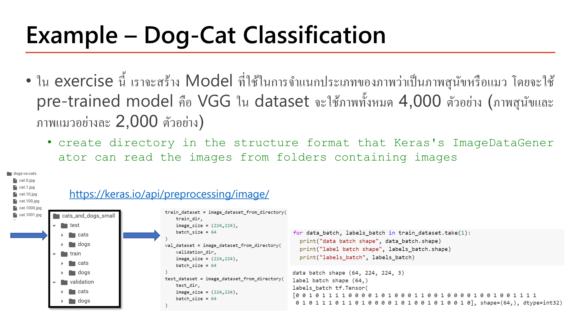
Slide: Example - Dog-Cat Classification. Build a model classifying dog or cat images using pretrained VGG; dataset of 4,000 images (2,000 dogs, 2,000 cats). Create directory structure cats_and_dogs_small with test, train, validation folders each containing cats and dogs. Code: train_dataset = image_dataset_from_directory(train_dir, image_size=(224,224), batch_size=64), same for validation and test. Output: data batch shape (64, 224, 224, 3), label batch shape (64,)
Slide: Example – Dog-Cat Classification — เตรียม dataset (Lecture8, p.26)

โจทย์: จำแนกภาพสุนัขหรือแมวด้วย pretrained model คือ VGG. Dataset มี 4,000 ภาพ (สุนัขและแมวอย่างละ 2,000). ขั้นแรกตามสไลด์คือ create directory in the structure format that Keras's ImageDataGenerator can read the images from folders containing images: โฟลเดอร์ cats_and_dogs_small มี train, validation, test และแต่ละโฟลเดอร์มีโฟลเดอร์ย่อย cats, dogs. ชื่อโฟลเดอร์ย่อยถูกใช้เป็น label.

train_dataset = image_dataset_from_directory(
    train_dir,
    image_size = (224,224),
    batch_size = 64
)
val_dataset = image_dataset_from_directory(
    validation_dir,
    image_size = (224,224),
    batch_size = 64
)
test_dataset = image_dataset_from_directory(
    test_dir,
    image_size = (224,224),
    batch_size = 64
)

for data_batch, labels_batch in train_dataset.take(1):
    print("data batch shape", data_batch.shape)
    print("label batch shape", labels_batch.shape)
    print("labels_batch", labels_batch)
โค้ดทำอะไร
image_dataset_from_directory(train_dir, ...)อ่านภาพจากโฟลเดอร์ แล้วกำหนด label จากชื่อโฟลเดอร์ย่อยตามลำดับตัวอักษร (cats = 0, dogs = 1)
image_size = (224,224)resize ทุกภาพเป็น 224×224 ซึ่งเป็นขนาดที่ VGG16 ใช้ในงานเดิม (guideline หน้า 23)
batch_size = 64dataset คืนข้อมูลทีละ 64 ภาพ
train_dataset.take(1)ดึง 1 batch มาตรวจ shape

ผลลัพธ์ที่พิมพ์ในสไลด์: data batch shape (64, 224, 224, 3), label batch shape (64,) และ labels_batch เป็น tensor ของ 0/1 จำนวน 64 ค่า (dtype=int32). Train set มี 2,000 ภาพ จึงมี \(\lceil 2000/64 \rceil = 32\) batch ต่อ epoch (31 batch เต็ม และ batch สุดท้าย \(2000 - 31 \times 64 = 16\) ภาพ).
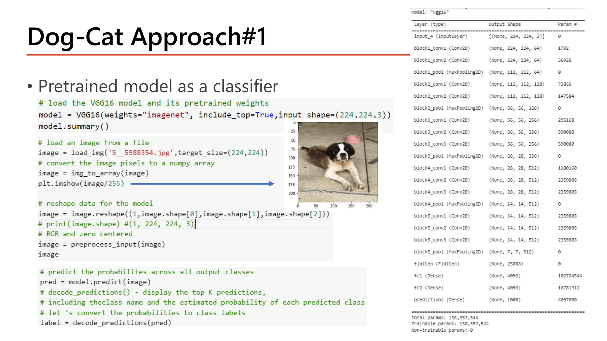
Slide: Dog-Cat Approach#1 Pretrained model as a classifier. Code: model = VGG16(weights="imagenet", include_top=True, input_shape=(224,224,3)); load_img with target_size=(224,224); img_to_array; reshape to (1, 224, 224, 3); preprocess_input; pred = model.predict(image); label = decode_predictions(pred). Model summary of vgg16 with fc1, fc2, predictions (None, 1000); Total params 138,357,544
Slide: Dog-Cat Approach#1 — Pretrained model as a classifier (Lecture8, p.27)

Approach #1: Pretrained model as a classifier. โหลด VGG16 ทั้งตัวรวม classifier 1,000 class แล้วทำนายทันที ไม่มีการเทรน.

# load the VGG16 model and its pretrained weights
model = VGG16(weights="imagenet", include_top=True,input_shape=(224,224,3))
model.summary()

# load an image from a file
image = load_img('S__5988354.jpg',target_size=(224,224))
# convert the image pixels to a numpy array
image = img_to_array(image)
plt.imshow(image/255)

# reshape data for the model
image = image.reshape((1,image.shape[0],image.shape[1],image.shape[2]))
# print(image.shape) #(1, 224, 224, 3)
# BGR and zero-centered
image = preprocess_input(image)
image

# predict the probabilites across all output classes
pred = model.predict(image)
# decode_predictions() - display the top K predictions,
# including theclass name and the estimated probability of each predicted class
# let 's convert the probabilities to class labels
label = decode_predictions(pred)
โค้ดทำอะไร
VGG16(weights="imagenet", include_top=True, input_shape=(224,224,3))โหลดสถาปัตยกรรม VGG16 พร้อม weight ที่เทรนบน ImageNet. include_top=True = รวม classifier (fc1, fc2, predictions) ไว้ด้วย
load_img(..., target_size=(224,224))โหลดภาพและ resize เป็นขนาดที่โมเดลต้องการ
img_to_array(image)แปลงเป็น numpy array shape (224, 224, 3) ค่า 0–255
image.reshape((1, image.shape[0], image.shape[1], image.shape[2]))เพิ่มมิติ batch ⇒ (1, 224, 224, 3). โมเดลรับ input เป็น batch เสมอ
preprocess_input(image)ปรับภาพแบบเดียวกับตอนเทรน VGG16: สลับ RGB เป็น BGR และลบค่าเฉลี่ยของแต่ละ channel (zero-centered)
model.predict(image)ได้ความน่าจะเป็น 1,000 ค่า shape (1, 1000)
decode_predictions(pred)แปลงเป็นชื่อ class พร้อมความน่าจะเป็นของ top K (default 5)
คำนวณตาม summary ในสไลด์: VGG16 มี 138,357,544 parameter อยู่ที่ไหน
ให้ ค่าจาก model.summary(): conv base ทั้งหมด (ถึง block5_pool) ให้ output (None, 7, 7, 512); fc1 และ fc2 มี 4,096 node; predictions มี 1,000 node
  1. ขั้นที่ 1 — block1_conv1 และ block1_conv2 (64 filter, 3×3)
    $$(3 \cdot 3 \cdot 3 + 1) \cdot 64 = 1{,}792 \qquad (3 \cdot 3 \cdot 64 + 1) \cdot 64 = 36{,}928$$
  2. ขั้นที่ 2 — Flatten แล้วเข้า fc1
    $$\begin{gathered}7 \times 7 \times 512 = 25{,}088 \\[0.35em] 25{,}088 \times 4{,}096 + 4{,}096 = 102{,}764{,}544\end{gathered}$$
  3. ขั้นที่ 3 — fc2 และ predictions
    $$\begin{gathered}4{,}096 \times 4{,}096 + 4{,}096 = 16{,}781{,}312 \\[0.35em] 4{,}096 \times 1{,}000 + 1{,}000 = 4{,}097{,}000\end{gathered}$$
  4. ขั้นที่ 4 — ส่วน conv base = ทั้งหมด − classifier
    $$\begin{gathered}138{,}357{,}544 - (102{,}764{,}544 + 16{,}781{,}312 + 4{,}097{,}000) \\[0.35em] = 14{,}714{,}688\end{gathered}$$

Classifier สาม dense layer มี 123.6 ล้าน parameter (89%) ส่วน convolution 13 ชั้นมีเพียง 14.7 ล้าน (11%). ค่า 14,714,688 คือ Total params ที่จะเห็นเมื่อโหลดด้วย include_top=False ใน approach #2. ข้อจำกัดของ approach #1: output เป็น 1,000 class ของ ImageNet (เช่น สายพันธุ์สุนัขและแมว) ไม่ใช่สอง class "dog/cat" ที่โจทย์ต้องการ.
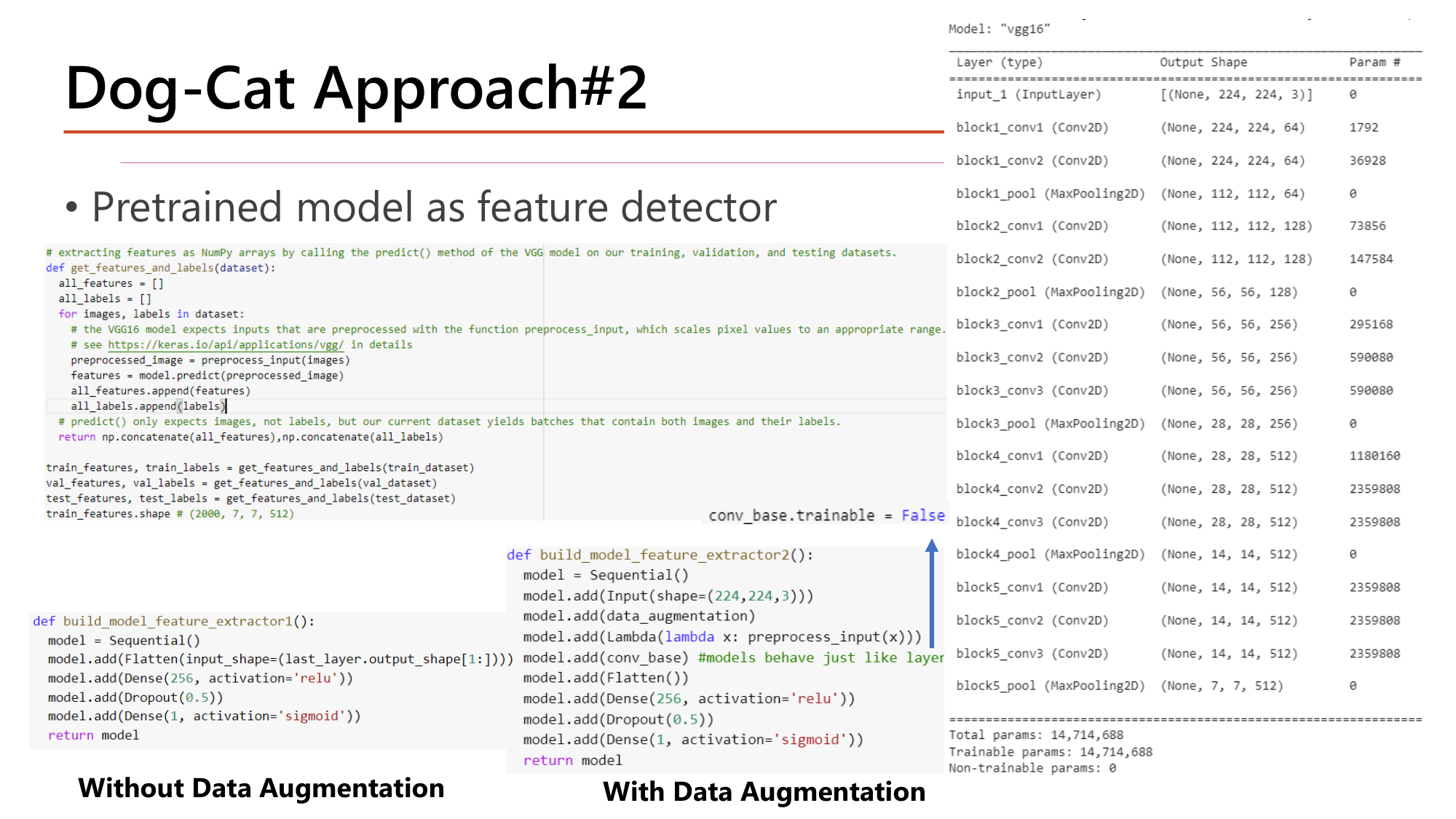
Slide: Dog-Cat Approach#2 Pretrained model as feature detector. Without data augmentation: get_features_and_labels(dataset) runs preprocess_input and conv_base.predict to extract features of shape (2000, 7, 7, 512); build_model_feature_extractor1: Flatten, Dense(256, relu), Dropout(0.5), Dense(1, sigmoid). With data augmentation: conv_base.trainable = False; build_model_feature_extractor2: Input(shape=(224,224,3)), data_augmentation, Lambda(preprocess_input), conv_base, Flatten, Dense(256), Dropout(0.5), Dense(1, sigmoid). vgg16 summary without top: Total params 14,714,688
Slide: Dog-Cat Approach#2 — Pretrained model as feature detector (Lecture8, p.28)

Approach #2: Pretrained model as feature detector. โหลดเฉพาะ conv base (include_top=False) แล้วต่อ classifier ใหม่. สไลด์แสดงสองวิธี.

วิธี A — Without Data Augmentation: ส่งภาพทั้งหมดผ่าน conv base ครั้งเดียวแล้วเก็บ feature เป็น array จากนั้นเทรน classifier เล็กๆ บน feature เหล่านั้น.

# instantiate the VGG16 model.
conv_base = VGG16(weights='imagenet',include_top=False,input_shape=(224,224,3))

# extracting features as NumPy arrays by calling the predict() method of the VGG model on our training, validation, and testing datasets.
def get_features_and_labels(dataset):
  all_features = []
  all_labels = []
  for images, labels in dataset:
    # the VGG16 model expects inputs that are preprocessed with the function preprocess_input, which scales pixel values to an appropriate range.
    preprocessed_image = preprocess_input(images)
    features = conv_base.predict(preprocessed_image)
    all_features.append(features)
    all_labels.append(labels)
  # predict() only expects images, not labels, but our current dataset yields batches that contain both images and their labels.
  return np.concatenate(all_features),np.concatenate(all_labels)

train_features, train_labels = get_features_and_labels(train_dataset)
val_features, val_labels = get_features_and_labels(val_dataset)
test_features, test_labels = get_features_and_labels(test_dataset)
train_features.shape # (2000, 7, 7, 512)

def build_model_feature_extractor1():
  model = Sequential()
  model.add(Flatten(input_shape=(last_layer.output_shape[1:])))
  model.add(Dense(256, activation='relu'))
  model.add(Dropout(0.5))
  model.add(Dense(1, activation='sigmoid'))
  return model
โค้ดทำอะไร
VGG16(weights='imagenet', include_top=False, input_shape=(224,224,3))include_top=False ตัด classifier (Flatten, fc1, fc2, predictions) ออก เหลือ conv base ที่จบที่ block5_pool. Total params 14,714,688
for images, labels in dataset:วนทีละ batch (64 ภาพ)
preprocess_input(images)ปรับ pixel ให้อยู่ในรูปแบบที่ VGG16 คาดหวัง
conv_base.predict(preprocessed_image)forward อย่างเดียว ไม่มีการเทรน. ได้ feature shape (64, 7, 7, 512) ต่อ batch
np.concatenate(all_features), np.concatenate(all_labels)ต่อทุก batch เป็น array เดียว ⇒ train_features.shape = (2000, 7, 7, 512)
Flatten(input_shape=(last_layer.output_shape[1:]))input ของโมเดลใหม่คือ feature (7, 7, 512) ไม่ใช่ภาพ. Flatten ได้ 25,088 ค่า
Dense(256, activation='relu') + Dropout(0.5)classifier ใหม่ที่เทรนจากศูนย์
Dense(1, activation='sigmoid')binary classification (dog/cat) ⇒ 1 node + sigmoid คู่กับ loss binary_crossentropy

วิธี B — With Data Augmentation: วิธี A ใช้ augmentation ไม่ได้ เพราะ feature ถูกคำนวณครั้งเดียวจากภาพเดิม. วิธี B จึงวาง conv base ไว้ในโมเดล เพื่อให้ภาพที่ถูก augment ใหม่ทุก epoch ไหลผ่าน conv base ทุกครั้ง และต้อง freeze conv base ด้วย conv_base.trainable = False.

conv_base.trainable = False

def build_model_feature_extractor2():
  model = Sequential()
  model.add(Input(shape=(224,224,3)))
  model.add(data_augmentation)
  model.add(Lambda(lambda x: preprocess_input(x)))
  model.add(conv_base) #models behave just like layers
  model.add(Flatten())
  model.add(Dense(256, activation='relu'))
  model.add(Dropout(0.5))
  model.add(Dense(1, activation='sigmoid'))
  return model
โค้ดทำอะไร
conv_base.trainable = Falsefreeze ทุก layer ของ conv base. ต้องทำก่อน compile
model.add(data_augmentation)pipeline ของ preprocessing layers จาก Lesson 7 §11
Lambda(lambda x: preprocess_input(x))ห่อ preprocess_input เป็น layer เพื่อให้อยู่ใน Sequential model ได้
model.add(conv_base)ใส่โมเดลทั้งตัวเป็น layer หนึ่งชั้น ("models behave just like layers")
Flatten → Dense(256) → Dropout(0.5) → Dense(1, sigmoid)classifier ชุดเดียวกับวิธี A
คำนวณ: trainable และ non-trainable parameter ของ approach #2 วิธี B
ให้ conv base ของ VGG16 มี 14,714,688 parameter และถูก freeze. Classifier: Flatten(7×7×512) → Dense(256) → Dense(1)
  1. ขั้นที่ 1 — Dense(256)
    $$25{,}088 \times 256 + 256 = 6{,}422{,}784$$
  2. ขั้นที่ 2 — Dense(1)
    $$256 \times 1 + 1 = 257$$
  3. ขั้นที่ 3 — Trainable = classifier ทั้งหมด
    $$6{,}422{,}784 + 257 = 6{,}423{,}041$$
  4. ขั้นที่ 4 — Total
    $$14{,}714{,}688 + 6{,}423{,}041 = 21{,}137{,}729$$

Total params 21,137,729; Trainable 6,423,041; Non-trainable 14,714,688. Dropout, Flatten, Lambda และ data augmentation ไม่มี parameter. วิธี A เทรนเร็วมาก (ราว 1 วินาทีต่อ epoch) เพราะเทรนเพียงสอง dense layer บน feature ที่คำนวณไว้แล้ว; วิธี B ช้ากว่าเพราะทุก batch ต้อง forward ผ่าน conv base. Test accuracy ที่ผู้สอนรันได้: วิธี A 0.974, วิธี B 0.980.
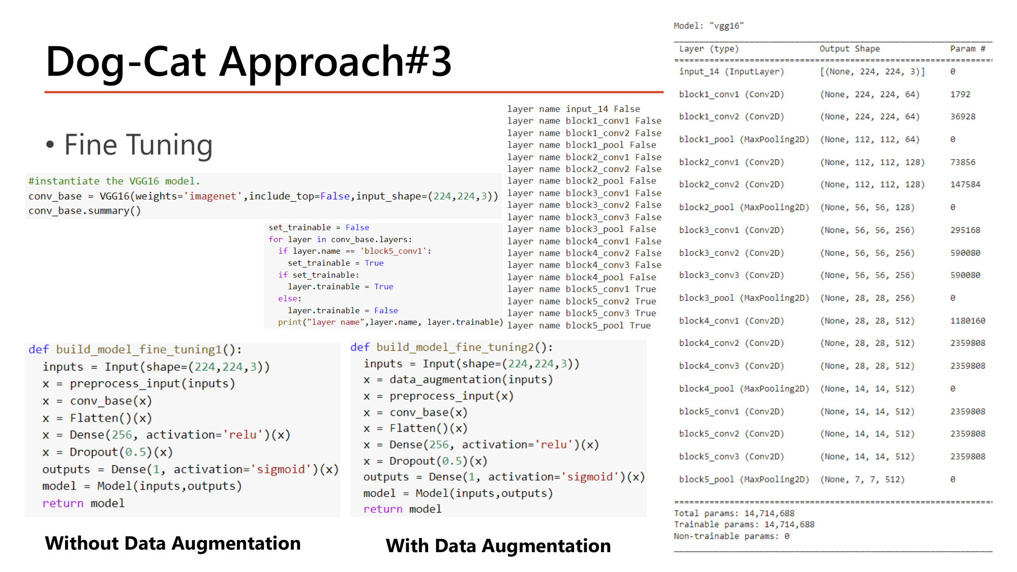
Slide: Dog-Cat Approach#3 Fine Tuning. conv_base = VGG16(weights='imagenet', include_top=False, input_shape=(224,224,3)). Loop: set_trainable = False; for layer in conv_base.layers: if layer.name == 'block5_conv1': set_trainable = True; layer.trainable set accordingly. Printout shows layers up to block4_pool False and block5_conv1, block5_conv2, block5_conv3, block5_pool True. build_model_fine_tuning1 (without augmentation) and build_model_fine_tuning2 (with augmentation) using the functional API
Slide: Dog-Cat Approach#3 — Fine Tuning (Lecture8, p.29)

Approach #3: Fine Tuning. freeze conv base ถึง block4 และปล่อย block5 (convolution สามชั้นสุดท้าย) ให้เทรนร่วมกับ classifier ใหม่.

#instantiate the VGG16 model.
conv_base = VGG16(weights='imagenet',include_top=False,input_shape=(224,224,3))
conv_base.summary()

set_trainable = False
for layer in conv_base.layers:
  if layer.name == 'block5_conv1':
    set_trainable = True
  if set_trainable:
    layer.trainable = True
  else:
    layer.trainable = False
  print("layer name",layer.name, layer.trainable)

def build_model_fine_tuning2():
  inputs = Input(shape=(224,224,3))
  x = data_augmentation(inputs)
  x = preprocess_input(x)
  x = conv_base(x)
  x = Flatten()(x)
  x = Dense(256, activation='relu')(x)
  x = Dropout(0.5)(x)
  outputs = Dense(1, activation='sigmoid')(x)
  model = Model(inputs,outputs)
  return model
โค้ดทำอะไร
set_trainable = Falseธงเริ่มต้น: layer ที่วนเจอก่อนถึงจุดตัดจะถูก freeze
for layer in conv_base.layers:วนตามลำดับจาก input ถึง block5_pool
if layer.name == 'block5_conv1': set_trainable = Trueเมื่อถึง block5_conv1 พลิกธงเป็น True และคงค่านั้นกับทุก layer ถัดไป
layer.trainable = True / Falseตั้งค่าของแต่ละ layer ตามธง
print("layer name", layer.name, layer.trainable)ผลลัพธ์: input ถึง block4_pool เป็น False; block5_conv1, block5_conv2, block5_conv3, block5_pool เป็น True
inputs = Input(shape=(224,224,3)) … model = Model(inputs, outputs)Functional API: เรียกแต่ละ layer เป็นฟังก์ชันบน tensor x แล้วสร้างโมเดลจาก input และ output. build_model_fine_tuning1 (without data augmentation) เหมือนกันแต่ไม่มีบรรทัด data_augmentation
คำนวณ: trainable parameter ของ approach #3
ให้ block5_conv1, block5_conv2, block5_conv3 มี 512 filter 3×3 และ input 512 channel. Classifier ชุดเดิม 6,423,041 parameter
  1. ขั้นที่ 1 — Convolution หนึ่งชั้นของ block5
    $$(3 \cdot 3 \cdot 512 + 1) \cdot 512 = 2{,}359{,}808$$
  2. ขั้นที่ 2 — สามชั้นที่ปลด freeze
    $$3 \times 2{,}359{,}808 = 7{,}079{,}424$$
  3. ขั้นที่ 3 — Trainable และ non-trainable
    $$\begin{gathered}7{,}079{,}424 + 6{,}423{,}041 = 13{,}502{,}465 \\[0.35em] 14{,}714{,}688 - 7{,}079{,}424 = 7{,}635{,}264\end{gathered}$$

Trainable 13,502,465; Non-trainable 7,635,264; Total 21,137,729 เท่า approach #2. ในแง่จำนวน layer: 4 จาก 19 layer ของ conv base ถูกปลด (ราว 21%) และ 79% ถูก freeze ซึ่งอยู่ในช่วง 60%–80% ของ scenario #2 เพราะ domain สุนัข/แมวคล้าย ImageNet มาก. ผู้สอน compile ด้วย Adam(learning_rate=0.00001) ซึ่งเล็กกว่า 0.001 ของ approach #2 ถึง 100 เท่า ตาม guideline หน้า 25. Test accuracy: without augmentation 0.972, with augmentation 0.980.

คำถาม 16Keras transfer learning
ต้องการโหลด VGG16 พร้อม weight ของ ImageNet โดยตัดส่วน fully connected classifier ออก เพื่อนำมาต่อ classifier ของตัวเอง ต้องเติมอาร์กิวเมนต์ใดในช่องว่างของ VGG16(weights='imagenet', ______, input_shape=(224,224,3))?
คำถาม 17Keras transfer learning
Conv base ที่ถูก freeze มี 14,714,688 parameter และให้ output 7×7×512 ต่อด้วย Flatten → Dense(128, relu) → Dropout(0.5) → Dense(1, sigmoid) โมเดลนี้มี trainable parameter กี่ตัว?
คำถาม 18Keras transfer learning
Train set มี 3,000 ภาพ โหลดด้วย image_dataset_from_directory(..., image_size=(224,224), batch_size=64) ข้อใดคือ shape ของ batch ข้อมูลหนึ่ง batch เต็ม และจำนวน batch ต่อ epoch?
ออกสอบสูง — โค้ดและตัวเลขของตัวอย่าง Dog-Cat

10. Beyond CNNs: Vision Transformer และ Swin Transformer

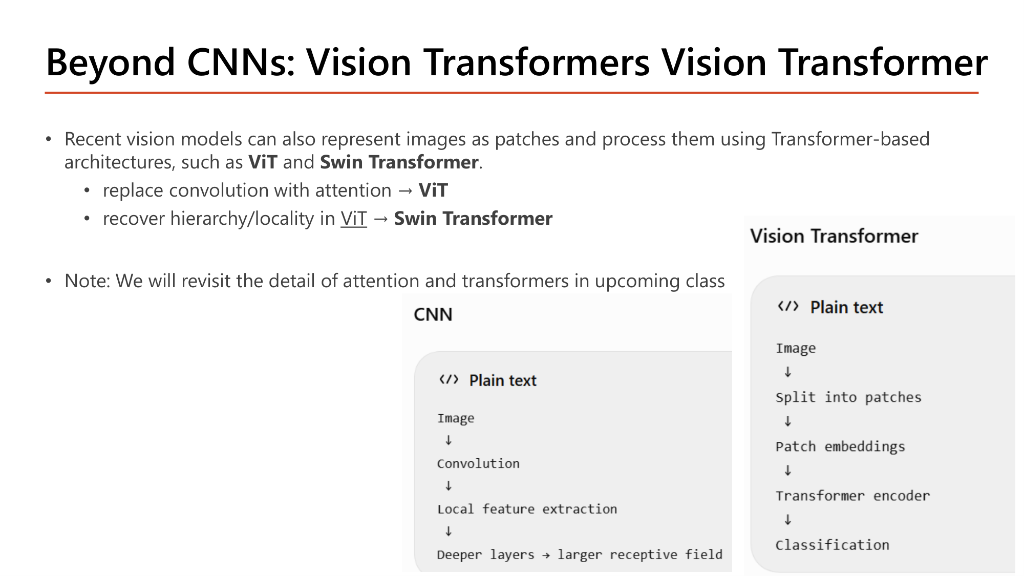
Slide: Beyond CNNs: Vision Transformers. Recent vision models can represent images as patches and process them using Transformer-based architectures such as ViT and Swin Transformer. Replace convolution with attention: ViT. Recover hierarchy/locality in ViT: Swin Transformer. CNN flow: image, convolution, local feature extraction, deeper layers with larger receptive field. Vision Transformer flow: image, split into patches, patch embeddings, transformer encoder, classification
Slide: Beyond CNNs: Vision Transformers — CNN เทียบกับ ViT (Lecture8, p.30)

โมเดล vision รุ่นใหม่แทนภาพเป็น patch แล้วประมวลผลด้วยสถาปัตยกรรมแบบ Transformer เช่น ViT และ Swin Transformer:

CNNVision Transformer
Image → Convolution → Local feature extraction → Deeper layers → larger receptive fieldImage → Split into patches → Patch embeddings → Transformer encoder → Classification

สไลด์หมายเหตุว่ารายละเอียดของ attention และ transformer จะเรียนในคาบถัดไป. ในบทนี้ให้เข้าใจ self-attention ว่าเป็นกลไกที่ทุก token คำนวณความสัมพันธ์กับ token อื่นแล้วรวมข้อมูลตามน้ำหนักความสัมพันธ์นั้น.
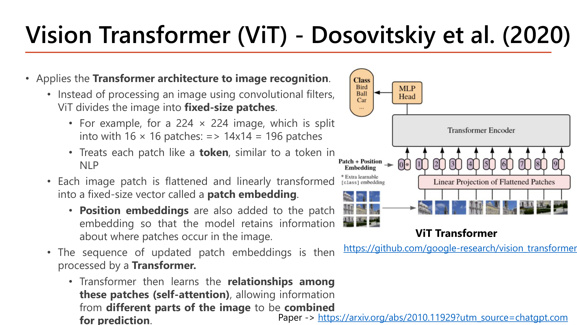
Slide: Vision Transformer (ViT), Dosovitskiy et al. (2020). Applies the Transformer architecture to image recognition. ViT divides the image into fixed-size patches; a 224x224 image with 16x16 patches gives 14x14 = 196 patches. Each patch is treated like a token, flattened and linearly transformed into a patch embedding; position embeddings are added; the sequence is processed by a Transformer that learns relationships among patches (self-attention). Diagram: patches, linear projection of flattened patches, patch + position embedding with extra class embedding, transformer encoder, MLP head, class
Slide: Vision Transformer (ViT) — patch และ embedding (Lecture8, p.31)

ViT (Dosovitskiy et al., 2020) ใช้ Transformer architecture to image recognition. ขั้นตอนตามสไลด์:

  1. แทนการใช้ convolutional filter ViT แบ่งภาพเป็น fixed-size patches และถือแต่ละ patch เป็น token เหมือน token ใน NLP
  2. แต่ละ patch ถูก flatten แล้วแปลงเชิงเส้นเป็น vector ขนาดคงที่ เรียกว่า patch embedding
  3. บวก position embeddings เข้ากับ patch embedding เพื่อให้โมเดลรู้ว่า patch อยู่ตรงไหนของภาพ
  4. ลำดับของ patch embedding ถูกประมวลผลด้วย Transformer ซึ่งเรียน relationships among these patches (self-attention) ทำให้ข้อมูลจาก different parts of the image ถูก combined for prediction
คำนวณตามสไลด์: จำนวน patch ของ ViT
ให้ ภาพ 224×224×3 แบ่งเป็น patch ขนาด 16×16
  1. ขั้นที่ 1 — จำนวน patch ต่อด้าน
    $$\frac{224}{16} = 14$$
  2. ขั้นที่ 2 — จำนวน patch ทั้งหมด
    $$14 \times 14 = 196 \text{ patches}$$
  3. ขั้นที่ 3 — ขนาดของ patch หนึ่งชิ้นหลัง flatten
    $$16 \times 16 \times 3 = 768 \text{ ค่า}$$
  4. ขั้นที่ 4 — จำนวนคู่ที่ global self-attention ต้องคำนวณ (ทุก patch กับทุก patch)
    $$196^2 = 38{,}416$$

ภาพหนึ่งภาพกลายเป็นลำดับ 196 token (รูปในสไลด์มี class embedding พิเศษอีก 1 ตัวที่ตำแหน่ง 0 สำหรับการจำแนก). ต้นทุนของ self-attention โตตามกำลังสองของจำนวน patch ซึ่งเป็นปัญหาที่ Swin แก้.
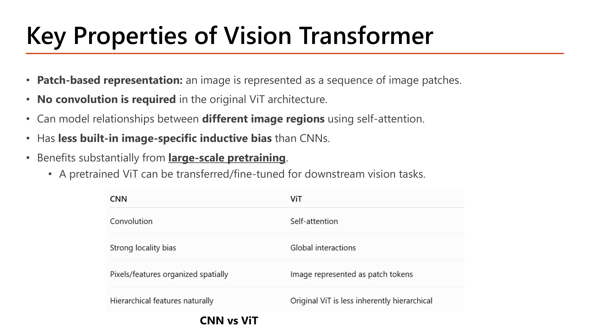
Slide: Key Properties of Vision Transformer. Patch-based representation; no convolution is required in the original ViT; can model relationships between different image regions using self-attention; has less built-in image-specific inductive bias than CNNs; benefits substantially from large-scale pretraining; a pretrained ViT can be transferred/fine-tuned for downstream tasks. Table CNN vs ViT: convolution vs self-attention; strong locality bias vs global interactions; pixels/features organized spatially vs image as patch tokens; hierarchical features naturally vs original ViT less inherently hierarchical
Slide: Key Properties of Vision Transformer — CNN vs ViT (Lecture8, p.32)
CNNViT
ConvolutionSelf-attention
Strong locality biasGlobal interactions
Pixels/features organized spatiallyImage represented as patch tokens
Hierarchical features naturallyOriginal ViT is less inherently hierarchical
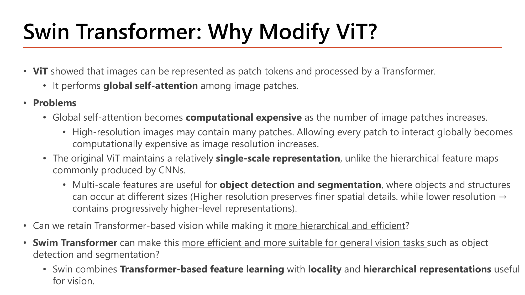
Slide: Swin Transformer: Why Modify ViT? ViT performs global self-attention among image patches. Problems: global self-attention becomes computationally expensive as the number of image patches increases (high-resolution images); the original ViT maintains a relatively single-scale representation, unlike hierarchical feature maps of CNNs; multi-scale features are useful for object detection and segmentation. Swin combines Transformer-based feature learning with locality and hierarchical representations
Slide: Swin Transformer: Why Modify ViT? (Lecture8, p.33)

ViT ทำ global self-attention ระหว่างทุก patch. สไลด์ระบุปัญหาสองข้อ:

  1. Global self-attention computational expensive เมื่อจำนวน patch เพิ่ม. ภาพความละเอียดสูงมี patch มาก การให้ทุก patch โต้ตอบกันทั้งหมดจึงแพงขึ้นตามความละเอียด
  2. ViT ดั้งเดิมคง single-scale representation ต่างจาก hierarchical feature map ของ CNN. Multi-scale feature มีประโยชน์กับ object detection and segmentation ที่วัตถุมีหลายขนาด (ความละเอียดสูงเก็บรายละเอียดเชิงพื้นที่; ความละเอียดต่ำเก็บ representation ระดับสูง)

คำถามที่ Swin ตอบ: คง vision แบบ Transformer ไว้โดยทำให้ more hierarchical and efficient ได้หรือไม่. Swin รวม Transformer-based feature learning กับ locality และ hierarchical representations.
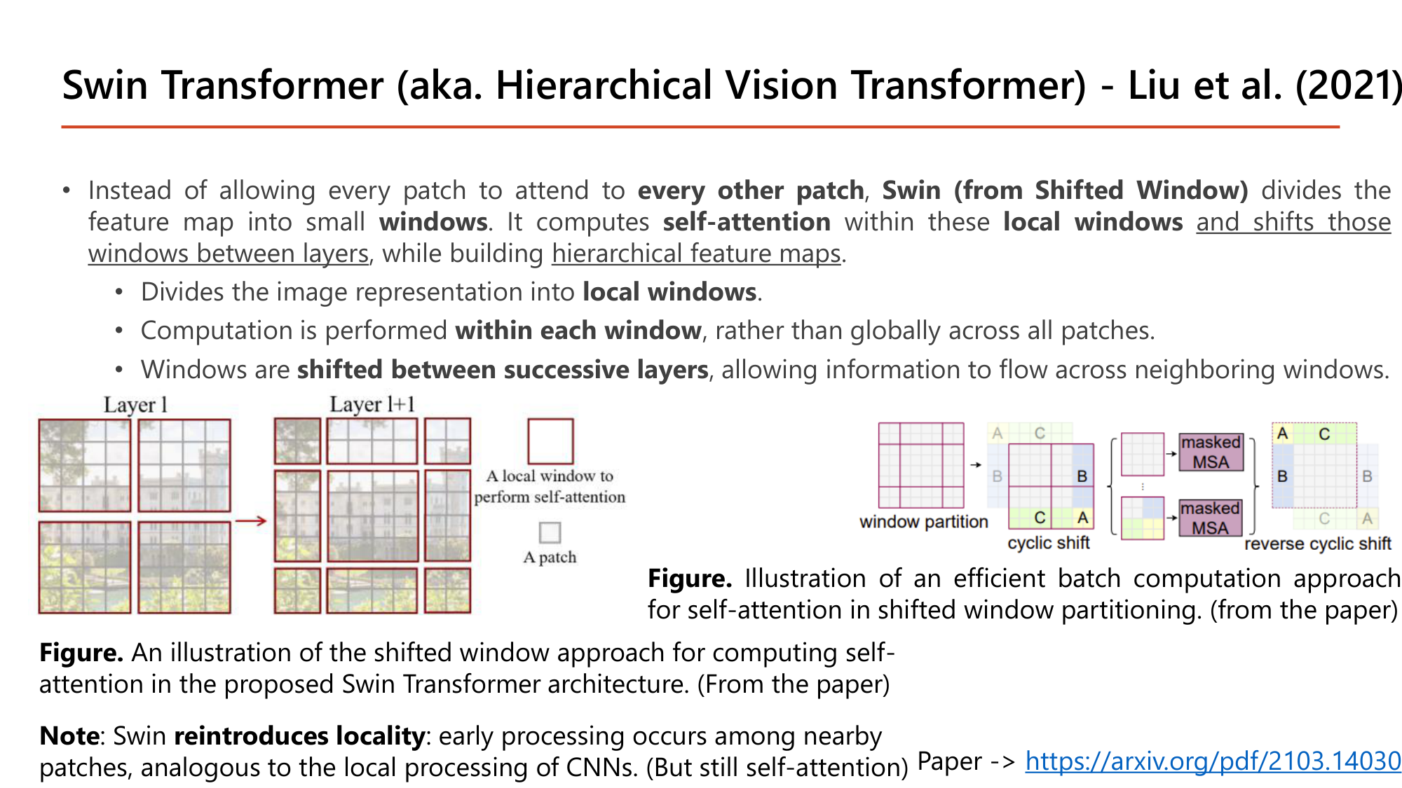
Slide: Swin Transformer (Hierarchical Vision Transformer), Liu et al. (2021). Instead of every patch attending to every other patch, Swin (Shifted Window) divides the feature map into small windows, computes self-attention within local windows and shifts the windows between layers, while building hierarchical feature maps. Figure: Layer l windows and Layer l+1 shifted windows. Note: Swin reintroduces locality, analogous to local processing of CNNs (but still self-attention)
Slide: Swin Transformer — shifted window (Lecture8, p.34)

แทนที่จะให้ทุก patch attend ไปยัง every other patch, Swin (from Shifted Window) แบ่ง feature map เป็น windows เล็กๆ. คำนวณ self-attention ภายใน local windows and shifts those windows between layers พร้อมสร้าง hierarchical feature maps:

รูปในสไลด์: Layer l แบ่งเป็น 4 window ปกติ. Layer l+1 เลื่อนขอบ window ไปครึ่งหนึ่ง patch ที่เคยอยู่คนละ window จึงมาอยู่ window เดียวกัน. หมายเหตุ: Swin reintroduces locality คือการประมวลผลช่วงต้นเกิดระหว่าง patch ใกล้กัน คล้าย local processing ของ CNN แต่ยังเป็น self-attention.

คำนวณ: global attention เทียบกับ window attention
ให้ feature map มี 14×14 = 196 patch. Swin ใช้ window ขนาด 7×7 patch
  1. ขั้นที่ 1 — Global attention (ViT)
    $$196^2 = 38{,}416 \text{ คู่}$$
  2. ขั้นที่ 2 — Window attention: จำนวน window และคู่ต่อ window
    $$\frac{196}{49} = 4 \text{ windows} \qquad 49^2 = 2{,}401 \text{ คู่ต่อ window}$$
  3. ขั้นที่ 3 — รวม
    $$4 \times 2{,}401 = 9{,}604 \text{ คู่}$$
  4. ขั้นที่ 4 — เพิ่มความละเอียดสองเท่าต่อด้าน (28×28 = 784 patch)
    $$\text{global: } 784^2 = 614{,}656 \qquad \text{window: } 16 \times 2{,}401 = 38{,}416$$

ที่ 196 patch window attention ถูกกว่า 4 เท่า. เมื่อ patch เพิ่ม 4 เท่า global attention แพงขึ้น 16 เท่า (กำลังสอง) แต่ window attention แพงขึ้นเพียง 4 เท่า (เชิงเส้น) ตรงกับแถว "High-resolution efficiency" ของตารางหน้า 36.
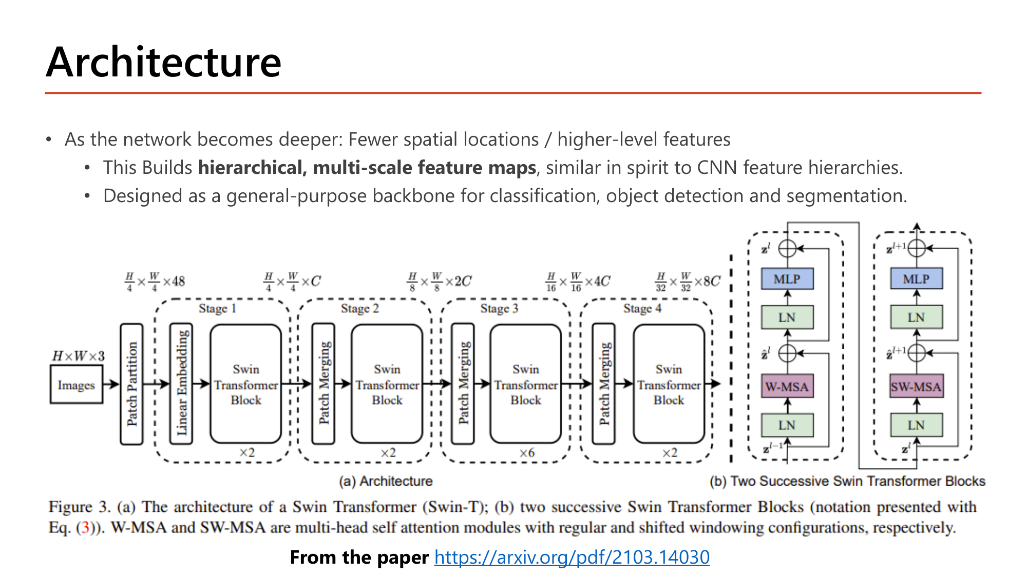
Slide: Architecture. As the network becomes deeper: fewer spatial locations / higher-level features. This builds hierarchical, multi-scale feature maps, similar in spirit to CNN feature hierarchies. Designed as a general-purpose backbone for classification, object detection and segmentation. Swin-T diagram: images HxWx3, patch partition H/4 x W/4 x 48, Stage 1 linear embedding and 2 Swin blocks H/4 x W/4 x C, Stage 2 patch merging and 2 blocks H/8 x W/8 x 2C, Stage 3 patch merging and 6 blocks H/16 x W/16 x 4C, Stage 4 patch merging and 2 blocks H/32 x W/32 x 8C; two successive Swin Transformer blocks with W-MSA and SW-MSA
Slide: Architecture — Swin-T สี่ stage (Lecture8, p.35)

เมื่อ network ลึกขึ้น: fewer spatial locations / higher-level features. สิ่งนี้สร้าง hierarchical, multi-scale feature maps คล้ายลำดับชั้น feature ของ CNN. Swin ออกแบบเป็น general-purpose backbone สำหรับ classification, object detection และ segmentation.

คำนวณตามรูปในสไลด์: ขนาด feature map ของ Swin-T แต่ละ stage
ให้ ภาพ 224×224×3 และ \(C = 96\). Patch partition ใช้ patch 4×4. Patch Merging ระหว่าง stage ลดด้านลงครึ่งและเพิ่ม channel สองเท่า
  1. ขั้นที่ 1 — Patch partition: patch 4×4 หนึ่งชิ้นมี \(4 \times 4 \times 3 = 48\) ค่า
    $$\frac{H}{4} \times \frac{W}{4} \times 48 = 56 \times 56 \times 48$$
  2. ขั้นที่ 2 — Stage 1 (Linear Embedding + 2 block)
    $$\frac{H}{4} \times \frac{W}{4} \times C = 56 \times 56 \times 96$$
  3. ขั้นที่ 3 — Stage 2 (Patch Merging + 2 block) และ Stage 3 (Patch Merging + 6 block)
    $$\begin{gathered}\frac{H}{8} \times \frac{W}{8} \times 2C = 28 \times 28 \times 192 \\[0.35em] \frac{H}{16} \times \frac{W}{16} \times 4C = 14 \times 14 \times 384\end{gathered}$$
  4. ขั้นที่ 4 — Stage 4 (Patch Merging + 2 block)
    $$\frac{H}{32} \times \frac{W}{32} \times 8C = 7 \times 7 \times 768$$

ลำดับ 56 → 28 → 14 → 7 พร้อม channel 96 → 192 → 384 → 768 คือรูปแบบ "เล็กลงแต่ลึกขึ้น" เดียวกับ CNN (VGG16: 112 → 56 → 28 → 14 → 7). Patch Merging ทำหน้าที่แทน pooling. ในรูป (b) บล็อกคู่ใช้ W-MSA (window ปกติ) แล้ว SW-MSA (shifted window) สลับกัน จำนวนบล็อกต่อ stage จึงเป็นเลขคู่ (2, 2, 6, 2).
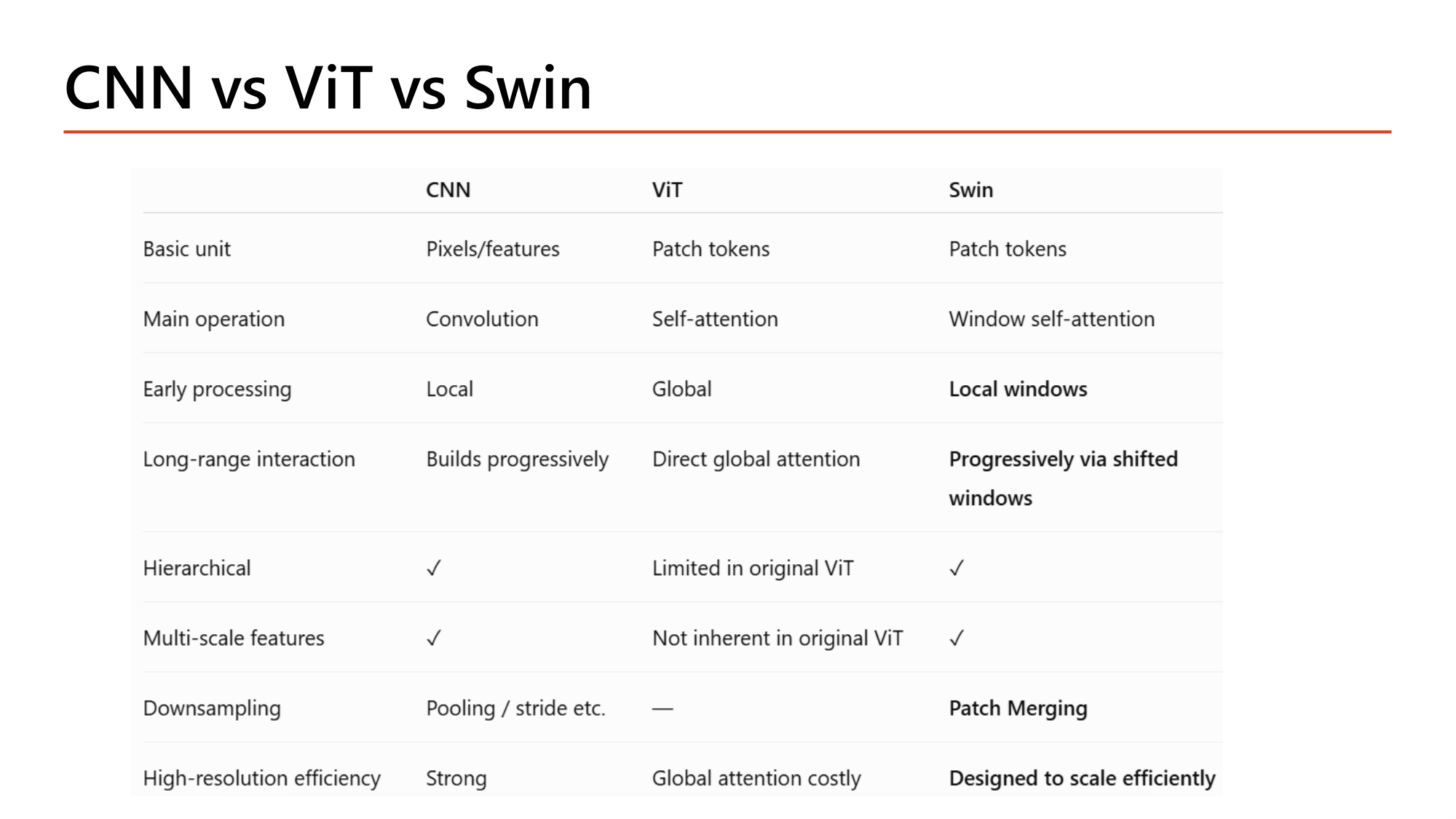
Slide: CNN vs ViT vs Swin table. Basic unit: pixels/features, patch tokens, patch tokens. Main operation: convolution, self-attention, window self-attention. Early processing: local, global, local windows. Long-range interaction: builds progressively, direct global attention, progressively via shifted windows. Hierarchical: yes, limited in original ViT, yes. Multi-scale features: yes, not inherent in original ViT, yes. Downsampling: pooling/stride, none, patch merging. High-resolution efficiency: strong, global attention costly, designed to scale efficiently
Slide: CNN vs ViT vs Swin — ตารางเปรียบเทียบ (Lecture8, p.36)
CNNViTSwin
Basic unitPixels/featuresPatch tokensPatch tokens
Main operationConvolutionSelf-attentionWindow self-attention
Early processingLocalGlobalLocal windows
Long-range interactionBuilds progressivelyDirect global attentionProgressively via shifted windows
Hierarchical✓Limited in original ViT✓
Multi-scale features✓Not inherent in original ViT✓
DownsamplingPooling / stride etc.—Patch Merging
High-resolution efficiencyStrongGlobal attention costlyDesigned to scale efficiently

อ่านตารางตามคอลัมน์: Swin ใช้ basic unit เดียวกับ ViT (patch tokens) แต่ในหกแถวที่เหลือมีคุณสมบัติตรงกับ CNN (local, progressive, hierarchical, multi-scale, มี downsampling, scale ได้). Swin จึงเป็น Transformer ที่นำข้อดีเชิงโครงสร้างของ CNN กลับมา.
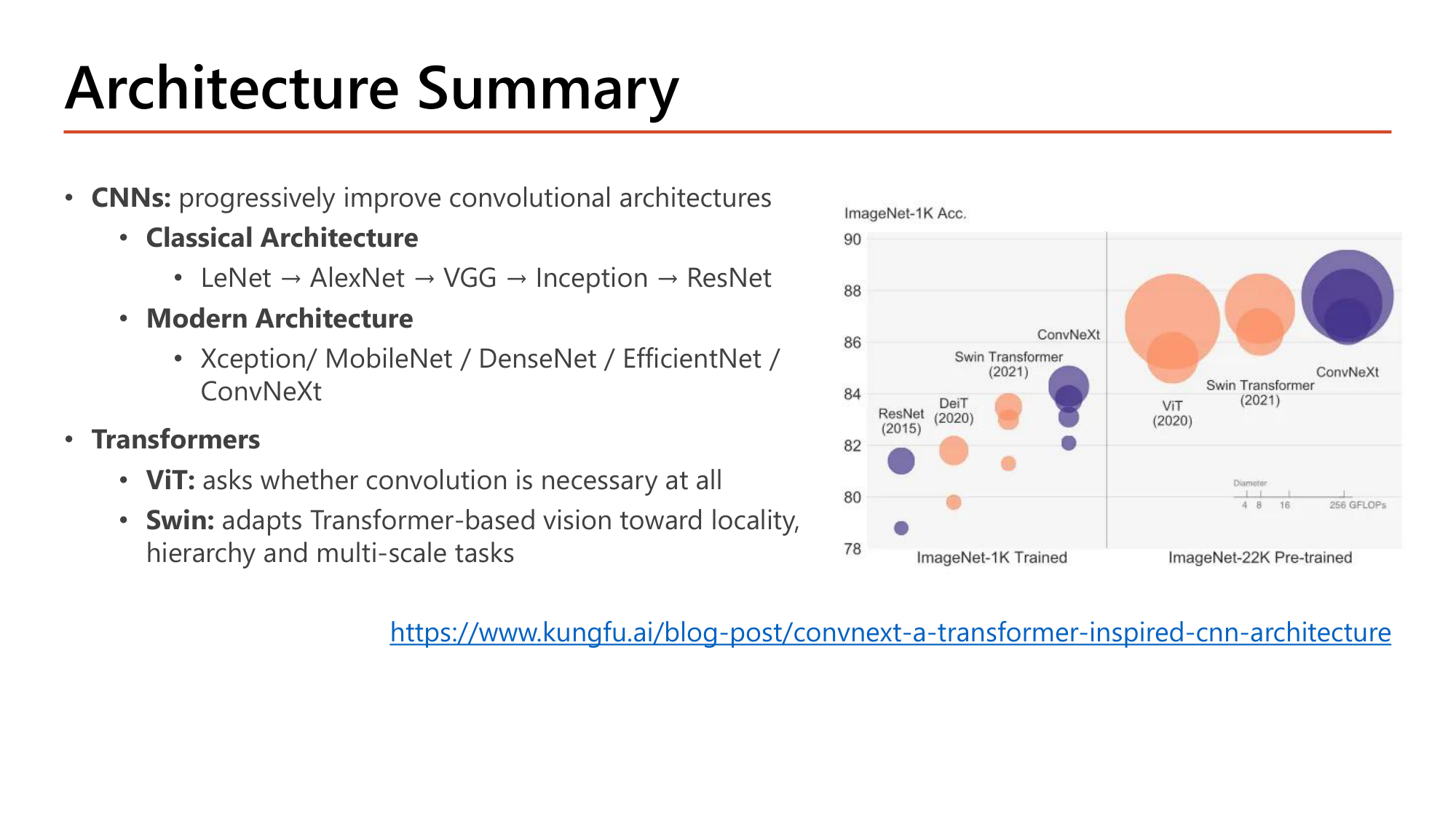
Slide: Architecture Summary. CNNs progressively improve convolutional architectures. Classical: LeNet, AlexNet, VGG, Inception, ResNet. Modern: Xception, MobileNet, DenseNet, EfficientNet, ConvNeXt. Transformers: ViT asks whether convolution is necessary at all; Swin adapts Transformer-based vision toward locality, hierarchy and multi-scale tasks. Chart of ImageNet-1K accuracy for ResNet, DeiT, Swin Transformer, ConvNeXt, ViT
Slide: Architecture Summary (Lecture8, p.37)

สรุปทั้งบทตามสไลด์:

กราฟในสไลด์แสดง ImageNet-1K accuracy: กลุ่มที่เทรนบน ImageNet-1K อยู่ช่วง 78–84% (ResNet ต่ำสุด, Swin และ ConvNeXt สูงสุด); กลุ่มที่ pretrain บน ImageNet-22K (ViT, Swin, ConvNeXt) ขึ้นไปถึง 85–88%. ทั้งสองข้อสอดคล้องกับที่สไลด์กล่าว: Transformer ได้ประโยชน์จาก large-scale pretraining และ ConvNeXt ซึ่งเป็น CNN ล้วนยังแข่งขันได้.

คำถาม 19ViT
ภาพขนาด 384×384 ถูกแบ่งเป็น patch ขนาด 32×32 โดย Vision Transformer จำนวน patch ทั้งหมดคือเท่าใด?
คำถาม 20ViT vs Swin
ข้อใดอธิบายความต่างของการคำนวณ self-attention ระหว่าง ViT ดั้งเดิมกับ Swin Transformer ได้ถูกต้อง?
คำถาม 21ViT vs CNN
ข้อใดเป็นคุณสมบัติของ Vision Transformer ดั้งเดิมเมื่อเทียบกับ CNN?
ออกสอบสูง — ข้อความที่อาจารย์ทำตัวหนา (หน้า 30–37 ไม่มีข้อความทำสี)


ชัยชนะของบทเรียนนี้
คุณควร (1) บอกได้ว่าแต่ละสถาปัตยกรรมแก้ปัญหาอะไร พร้อมตัวเลขคู่ จำนวน layer / top-5 error (8 / 15.3%, 16 / 7.3%, 22 / 6.67%, 152 / 4.49%); (2) คำนวณขนาด feature map ของ AlexNet (227 → 55 → 27 → 13 → 6) และ parameter ของ LeNet-5 (61,706); (3) แสดงด้วยตัวเลขว่า 3×3 ซ้อนกันประหยัดกว่า kernel ใหญ่ (73,856 เทียบกับ 102,464) และ 1×1 bottleneck ลดการคูณจาก 120,422,400 เหลือ 12,443,648; (4) อธิบาย \(h(x) = f(x) + x\) และนับ layer ของ ResNet-34/50/152; (5) คำนวณ parameter ของ depthwise separable convolution (8,896 เทียบกับ 73,856); (6) เลือกระดับ transfer learning จากขนาด dataset และความคล้ายของ domain และเขียนโค้ด VGG16 ทั้งสามแนวทาง พร้อมคำนวณ trainable parameter (6,423,041 และ 13,502,465); (7) คำนวณจำนวน patch ของ ViT (196) และเทียบ CNN / ViT / Swin ได้ครบแปดแถว.

ภาคผนวก: Slide ทั้งหมดใน deep_learning_part3_2.pdf (37 หน้า) — เช็คว่าอ่านครบ

หน้าเนื้อหาสถานะ
1ปก Part 3 — Convolutional Neural Network & Transfer Learningetc — สไลด์ปก (ชื่อวิชา, ภาคเรียน, เวลาเรียน) ไม่มีเนื้อหาวิชา
2Evolution of CNN Architectures✓ หัวข้อ 1 (รูป + ตารางแผนที่)
3Classical CNN Architectures / ILSVRC✓ หัวข้อ 1 (รูป + ตารางผู้ชนะ)
4LeNet-5✓ หัวข้อ 2 (รูป + คำนวณ 61,706)
5AlexNet✓ หัวข้อ 3 (รูป + คำนวณ 227→55→27→13→6)
6AlexNet Key Takeaways✓ หัวข้อ 3 (รูป + โค้ด Keras)
7VGGNet✓ หัวข้อ 4 (รูป + รูปแบบ channel)
8VGGNet Key Takeaways✓ หัวข้อ 4 (รูป + คำนวณ 3×3 เทียบ 5×5)
9Inception and GoogLeNet✓ หัวข้อ 5 (รูป + การทำงานของโมดูล)
10Computational Cost of Naive Inception Module✓ หัวข้อ 5 (รูป + คำนวณเต็ม + แก้ตัวเลขพิมพ์ผิด)
11GoogLeNet Architecture✓ หัวข้อ 5 (รูป + คำนวณ 256/480)
12Inception Key Takeaways✓ หัวข้อ 5 (รูป + สามข้อสรุป)
13ResNet (Residual Network)✓ หัวข้อ 6 (รูป + h(x) = f(x) + x)
14ResNet Architecture✓ หัวข้อ 6 (รูป + นับ layer 34/50/152)
15ResNet Key Takeaways✓ หัวข้อ 6 (รูป + ตาราง 5 รุ่น)
16Comparison✓ หัวข้อ 6 (รูป + ตาราง + อัตราส่วน)
17Modern CNNs✓ หัวข้อ 7 (รูป + ตาราง 5 รุ่น)
18Xception✓ หัวข้อ 7 (รูป + คำนวณ separable)
19Other Noteworthy Architectures✓ หัวข้อ 7 (รูป + ตาราง + ตัวอย่าง DenseNet)
20Architecture Design✓ หัวข้อ 7 (รูป + หลักออกแบบ)
21Transfer Learning✓ หัวข้อ 8 (รูป + Model A/B)
22Transfer Learning Approaches✓ หัวข้อ 8 (รูป + ตารางสามแนวทาง)
23Transfer Learning Guidelines✓ หัวข้อ 8 (รูป + input/hidden/output)
24Transfer Learning Guidelines (2)✓ หัวข้อ 8 (รูป + ตารางสี่ scenario)
25Transfer Learning Guidelines (3)✓ หัวข้อ 8 (รูป + ลำดับการเทรน)
26Example – Dog-Cat Classification✓ หัวข้อ 9 (รูป + โค้ด + คำนวณ batch)
27Dog-Cat Approach#1✓ หัวข้อ 9 (รูป + โค้ด + คำนวณ 138,357,544)
28Dog-Cat Approach#2✓ หัวข้อ 9 (รูป + โค้ดสองวิธี + คำนวณ 6,423,041)
29Dog-Cat Approach#3✓ หัวข้อ 9 (รูป + โค้ด + คำนวณ 13,502,465)
30Beyond CNNs: Vision Transformers✓ หัวข้อ 10 (รูป + CNN เทียบ ViT)
31Vision Transformer (ViT)✓ หัวข้อ 10 (รูป + คำนวณ 196 patch)
32Key Properties of Vision Transformer✓ หัวข้อ 10 (รูป + ตาราง)
33Swin Transformer: Why Modify ViT?✓ หัวข้อ 10 (รูป + สองปัญหา)
34Swin Transformer✓ หัวข้อ 10 (รูป + คำนวณ window attention)
35Architecture (Swin-T)✓ หัวข้อ 10 (รูป + คำนวณสี่ stage)
36CNN vs ViT vs Swin✓ หัวข้อ 10 (รูป + ตารางแปดแถว)
37Architecture Summary✓ หัวข้อ 10 (รูป + สรุป)

สงสัยตรงไหน ถามได้เลยในแชท — ผมเป็นผู้สอนของคุณ ถามซ้ำได้ ถามลึกได้ ไม่ต้องเกรงใจ.